Getting started

In order to start using SCRIMP, you have to work in the conda environment scrimp from the installation by running conda activate scrimp.

To understand the coding philosophy of SCRIMP, let us consider the 1D wave equation with Neumann boundary control as a first example

\[\begin{split}\left\lbrace \begin{array}{rcl} \rho(x) \partial_{tt}^2 w(t,x) - \partial_x \left( T(x) \partial_x w(t,x) \right) &=& 0, \qquad t \ge 0, x \in (0,1), \\ \partial_t w(0,x) &=& v_0(x), \qquad x \in (0,1), \\ \partial_x w(0,x) &=& s_0(x), \qquad x \in (0,1), \\ - T(0) \partial_x \left( w(t,0) \right) &=& u_L(t), \qquad t \ge 0, \\ T(1) \partial_x \left( w(t,1) \right) &=& u_R(t), \qquad t \ge 0, \end{array} \right.\end{split}\]

where \(w\) denotes the deflection from the equilibrium position of a string, \(\rho\) is its mass density and \(T\) the Young’s modulus. Note the minus sign on the control at the left end side, standing for the outward normal to the domain \((0,1)\).

The physics giving this equation has to be restated in the port-Hamiltonian formalism first.

Port-Hamiltonian framework

Let \(\alpha_q := \partial_x w\) denotes the strain and \(\alpha_p := \rho \partial_t w\) the linear momentum. One can express the total mechanical energy lying in the system \(\mathcal{H}\), the Hamiltonian, as

\[\mathcal{H}(t) = \mathcal{H}(\alpha_q(t,x), \alpha_p(t,x)) := \underbrace{\frac{1}{2} \int_0^1 \alpha_q(t,x) T(x) \alpha_q(t,x) {\rm d}x}_{\text{Potential energy}} + \underbrace{\frac{1}{2} \int_0^1 \frac{\alpha_p(t,x)^2}{\rho(x)} {\rm d}x}_{\text{Kinetic energy}}.\]

The variables \(\alpha_q\) and \(\alpha_p\) are known as the state variables, or in the present case since \(\mathcal{H}\) represents an energy, the energy variables.

Computing the variational derivative of \(\mathcal{H}\) with respect to these variables leads to the co-state variables, or in our case the co-energy variables, i.e.

\[e_q := \delta_{\alpha_q} \mathcal{H} = T \alpha_q, \qquad e_p := \delta_{\alpha_p} \mathcal{H} = \frac{\alpha_p}{\rho},\]

that is the stress and the velocity respectively.

Newton’s second law and Schwarz’s lemma give the following dynamics

\[\begin{split}\begin{pmatrix} \partial_t \alpha_q \\ \partial_t \alpha_p \end{pmatrix} = \begin{bmatrix} 0 & \partial_x \\ \partial_x & 0 \end{bmatrix} \begin{pmatrix} e_q \\ e_p \end{pmatrix}.\end{split}\]

Of course, trivial substitutions in this system would lead again to the initial string equation in second-order form. However, by keeping the system as is, an important structure appears. Indeed, the matrix of operators above is formally skew-symmetric. In other words, for all test functions \(f_q\) and \(f_p\) (compactly supported \(C^\infty\) functions), one has thanks to integration by parts

\[\begin{split}\begin{pmatrix} f_q & f_p \end{pmatrix} \begin{bmatrix} 0 & \partial_x \\ \partial_x & 0 \end{bmatrix} \begin{pmatrix} f_q \\ f_p \end{pmatrix} = 0.\end{split}\]

Together with the boundary Neumann condition, and defining collocated Dirichlet observations, this defines a (Stokes-) Dirac structure, where solutions along time, i.e. trajectories, will belong.

The port-Hamiltonian system representing a (linear) vibrating string with Neumann boundary control and Dirichlet boundary observation then writes

\[\begin{split}\begin{pmatrix} \partial_t \alpha_q \\ \partial_t \alpha_p \end{pmatrix} = \begin{bmatrix} 0 & \partial_x \\ \partial_x & 0 \end{bmatrix} \begin{pmatrix} e_q \\ e_p \end{pmatrix},\end{split}\]

\[\begin{split}\left\lbrace \begin{array}{rcl} - e_q(t,0) &=& u_L(t), \\ e_q(t,1) &=& u_R(t), \\ y_L(t) &=& e_p(t,0), \\ y_R(t) &=& e_p(t,1), \end{array} \right.\end{split}\]

\[\begin{split}\left\lbrace \begin{array}{rcl} e_q &=& T \alpha_q, \\ e_p &=& \frac{\alpha_p}{\rho}. \end{array} \right.\end{split}\]

The two first blocks, giving in particular the dynamics, define the Dirac structure of the system. The third block is known as the constitutive relations, and is needed to ensure uniqueness of solutions.

The importance of the Dirac structure relies, in particular, in the fact that it encloses the power balance satisfied by the Hamiltonian. Indeed, along the trajectories, one has

\[\frac{\rm d}{{\rm d}t} \mathcal{H}(t) = \frac{\rm d}{{\rm d}t} \mathcal{H}(\alpha_q(t), \alpha_p(t)) = \underbrace{y_R(t) u_R(t)}_{\text{power flowing through the right}} + \underbrace{y_L(t) u_L(t)}_{\text{power flowing through the left}}.\]

In other words, the Dirac structure encodes the way the system communicates with its environment. In the present example, it says that the variation of the total mechanical energy is given by the power supplied to the system at the boundaries.

Each couple \((\partial_t \alpha_q, e_q)\), \((\partial_t \alpha_p, e_p)\), \((u_L, y_L)\) and \((u_R, y_R)\) is a port of the port-Hamiltonian system, and is associated to a physically meaningful term in the power balance.

Structure-preserving discretization

The objective of a structure-preserving discretization method is to obtain a finite-dimensional Dirac structure that encloses a discrete version of the power balance. There is several ways to achieve this goal, but SCRIMP focuses on a particular application of the Mixed Finite Element Mehod, called the Partitioned Finite Element Method.

Remark: The 1D case does simplify the difficulties coming from the boundary terms. Indeed, here the functional spaces for the controls \(u_L\), \(u_R\) and the observations \(y_L\), \(y_R\) are nothing but \(\mathbb{R}\).

Let \(\varphi_q\) and \(\varphi_p\) be smooth test functions, and \(\delta_{mx}\) denote the Kronecker symbol. One can write the weak formulation of the Dirac Structure as follows

\[\begin{split}\left\lbrace \begin{array}{rcl} \int_0^1 \partial_t \alpha_q(t,x) \varphi_q(x) {\rm d}x &=& \int_0^1 \partial_x e_p(t,x) \varphi_q(x) {\rm d}x, \\ \int_0^1 \partial_t \alpha_p(t,x) \varphi_p(x) {\rm d}x &=& \int_0^1 \partial_x e_q(t,x) \varphi_p(x) {\rm d}x, \\ y_L(t) &=& \delta_{0x} e_p(t,x), \\ y_R(t) &=& \delta_{1x} e_p(t,x). \end{array} \right.\end{split}\]

Integrating by parts the second line make the controls appear

\[\begin{split}\left\lbrace \begin{array}{rcl} \int_0^1 \partial_t \alpha_q(t,x) \varphi_q(x) {\rm d}x &=& \int_0^1 \partial_x e_p(t,x) \varphi_q(x) {\rm d}x, \\ \int_0^1 \partial_t \alpha_p(t,x) \varphi_p(x) {\rm d}x &=& - \int_0^1 e_q(t,x) \partial_x \varphi_p(x) {\rm d}x + u_R(t) \varphi_p(1) + u_L(t) \varphi_p(0), \\ y_L(t) &=& \delta_{0x} e_p(t,x), \\ y_R(t) &=& \delta_{1x} e_p(t,x). \end{array} \right.\end{split}\]

Now, let \((\varphi_q^i)_{1 \le i \le N_q}\) and \((\varphi_p^k)_{1 \le k \le N_p}\) be two finite families of approximations for the \(q\)-type port and the \(p\)-type port respectively, typically finite element families, and write the discrete weak formulation with those families, one has for all \(1 \le i \le N_q\) and all \(1 \le k \le N_p\)

\[\begin{split}\left\lbrace \begin{array}{rcl} \sum_{j=1}^{N_q} \int_0^1 \varphi_q^j(x) \varphi_q^i(x) {\rm d}x \, \frac{\rm d}{{\rm d}t} \alpha_q^j(t) &=& \sum_{\ell=1}^{N_p} \int_0^1 \partial_x \varphi_p^\ell(x) \varphi_q^i(x) {\rm d}x \, e_p^\ell(t), \\ \sum_{\ell=1}^{N_p} \int_0^1 \varphi_p^\ell(x) \varphi_p^k(x) {\rm d}x \, \frac{\rm d}{{\rm d}t} \alpha_p^\ell(t) &=& - \sum_{j=1}^{N_q} \int_0^1 \varphi_q^j(x) \partial_x \varphi_p^k(x) {\rm d}x \, e_q^j(t) \\ && \qquad \qquad + u_R(t) \varphi_p^k(1) + u_L(t) \varphi_p^k(0), \\ y_L(t) &=& \sum_{\ell=1}^{N_p} \varphi_p^\ell(0) \, e_p^\ell(t), \\ y_R(t) &=& \sum_{\ell=1}^{N_p} \varphi_p^\ell(1) \, e_p^\ell(t), \end{array} \right.\end{split}\]

which rewrites in matrix form

\[\begin{split}\underbrace{\begin{bmatrix} M_q & 0 & 0 & 0 \\ 0 & M_p & 0 & 0 \\ 0 & 0 & 1 & 0 \\ 0 & 0 & 0 & 1 \end{bmatrix}}_{= M} \begin{pmatrix} \frac{\rm d}{{\rm d}t} \underline{\alpha_q}(t) \\ \frac{\rm d}{{\rm d}t} \underline{\alpha_p}(t) \\ - y_L(t) \\ - y_R(t) \end{pmatrix} = \underbrace{\begin{bmatrix} 0 & D & 0 & 0 \\ -D^\top & 0 & B_L & B_R \\ 0 & -B_L^\top & 0 & 0 \\ 0 & -B_R^\top & 0 & 0 \end{bmatrix}}_{= J} \begin{pmatrix} \underline{e_q}(t) \\ \underline{e_p}(t) \\ u_L(t) \\ u_R(t) \end{pmatrix},\end{split}\]

where \(\underline{\alpha_\star}(t) := \begin{pmatrix} \alpha_\star^1(t) & \cdots & \alpha_\star^{N_\star} \end{pmatrix}^\top\), \(\underline{e_\star}(t) := \begin{pmatrix} e_\star^1(t) & \cdots & e_\star^{N_\star} \end{pmatrix}^\top\), and

\[(M_q)_{ij} := \int_0^1 \varphi_q^j(x) \varphi_q^i(x) {\rm d}x, \qquad (M_p)_{k\ell} := \int_0^1 \varphi_p^\ell(x) \varphi_p^k(x) {\rm d}x,\]

\[(D)_{i\ell} := \int_0^1 \partial_x \varphi_p^\ell(x) \varphi_q^i(x) {\rm d}x, \qquad (B_L)_{k} := \varphi_p^k(0), \qquad (B_R)_{k} := \varphi_p^k(1).\]

Abusing the language, the left-hand side will be called the flow of the Dirac structure in SCRIMP, while the right-hand side will be called the effort.

Now one can approximate the constitutive relations in those families by projection of their weak formulations

\[\begin{split}\left\lbrace \begin{array}{rcl} \int_0^1 e_q(t,x) \varphi_q(x) {\rm d}x &=& \int_0^1 T(x) \alpha_q(t,x) \varphi_q(x) {\rm d}x, \\ \int_0^1 e_p(t,x) \varphi_p(x) {\rm d}x &=& \int_0^1 \frac{\alpha_p(t,x)}{\rho(x)} \varphi_p(x) {\rm d}x, \end{array} \right.\end{split}\]

from which one can deduce the matrix form of the discrete weak formulation of the constitutive relation

\[\begin{split}\left\lbrace \begin{array}{rcl} M_q \underline{e_q}(t) &=& M_T \underline{\alpha_q}(t), \\ M_p \underline{e_p}(t) &=& M_\rho \underline{\alpha_p}(t), \end{array} \right.\end{split}\]

where

\[(M_T)_{ij} := \int_0^1 T(x) \varphi_q^j(x) \varphi_q^i(x) {\rm d}x, \qquad (M_\rho)_{k\ell} := \int_0^1 \frac{\varphi_p^\ell(x)}{\rho(x)} \varphi_p^k(x) {\rm d}x.\]

Finally, the discrete Hamiltonian \(\mathcal{H}^d\) is defined as the evaluation of \(\mathcal{H}\) on the approximation of the state variables

\[\mathcal{H}^d(t) := \mathcal{H}(\alpha_q^d(t,x), \alpha_p^d(t)) = \frac{1}{2} \underline{\alpha_q}(t)^\top M_T \underline{\alpha_q}(t) + \frac{1}{2} \underline{\alpha_p}(t)^\top M_\rho \underline{\alpha_p}(t).\]

The discrete power balance is then easily deduced from the above matrix formulations, thanks to the symmetry of \(M\) and the skew-symmetry of \(J\)

\[\frac{\rm d}{{\rm d}t} \mathcal{H}^d(t) = y_R(t) u_R(t) + y_L(t) u_L(t).\]

Remark: The discrete system that has to be solved numerically is a Differential Algebraic Equation (DAE). There exists some case (as in this example), where one can write the co-state formulation of the system by substituting the constitutive relations at the continuous level to get a more classical Ordinary Differential Equation (ODE)

\[\begin{split}\begin{bmatrix} \widetilde{M}_q & 0 & 0 & 0 \\ 0 & \widetilde{M}_p & 0 & 0 \\ 0 & 0 & 1 & 0 \\ 0 & 0 & 0 & 1 \end{bmatrix} \begin{pmatrix} \frac{\rm d}{{\rm d}t} \underline{e_q}(t) \\ \frac{\rm d}{{\rm d}t} \underline{e_p}(t) \\ - y_L(t) \\ - y_R(t) \end{pmatrix} = \begin{bmatrix} 0 & D & 0 & 0 \\ -D^\top & 0 & B_L & B_R \\ 0 & -B_L^\top & 0 & 0 \\ 0 & -B_R^\top & 0 & 0 \end{bmatrix} \begin{pmatrix} \underline{e_q}(t) \\ \underline{e_p}(t) \\ u_L(t) \\ u_R(t) \end{pmatrix},\end{split}\]

where this time the mass matrices on the left-hand side are both weighted with respect to the physical parameters

\[(\widetilde{M}_q)_{ij} := \int_0^1 T^{-1}(x) \varphi_q^j(x) \varphi_q^i(x) {\rm d}x, \qquad (\widetilde{M}_p)_{k\ell} := \int_0^1 \rho(x) \varphi_p^\ell(x) \varphi_p^k(x) {\rm d}x.\]

Coding within SCRIMP

The following code is available in the file wave_1D.py of the sandbox folder of scrimp.

To start, import SCRIMP and create a distributed port-Hamiltonian system (DPHS) called, e.g., wave

import scrimp as S

wave = S.DPHS("real")

Then, define the domain \(\Omega = (0,1)\), with a mesh-size parameter \(h\), and add it to the DPHS

domain = S.Domain("Interval", {"L": 1., "h": 0.01})
wave.set_domain(domain)

This creates a mesh of the interval \(\Omega = (0,1)\).

Important to keep in mind: the domain is composed of regions, denoted by integers. The built-in geometry of an interval available in the code returns 1 for the domain \(\Omega\), 10 for the left-end and 11 for the right-end. Informations about available geometries and the indices of their regions can be found in the documentation or via the function built_in_geometries() available in scrimp.utils.mesh.

On this domain, we define two states and add them to the DPHS

alpha_q = S.State("q", "Strain", "scalar-field")
alpha_p = S.State("p", "Linear momentum", "scalar-field")
wave.add_state(alpha_q)
wave.add_state(alpha_p)

and the two associated co-states

e_q = S.CoState("e_q", "Stress", alpha_q)
e_p = S.CoState("e_p", "Velocity", alpha_p)
wave.add_costate(e_q)
wave.add_costate(e_p)

These latter calls create automatically two non-algebraic ports, named after their respective state. Note that we simplify the notations and do not write alpha_q and alpha_p but q and p for the sake of readability.

Finally, we create and add the two control-observation ports with

left_end = S.Control_Port("Boundary control (left)", "U_L", "Normal force", "Y_L", "Velocity", "scalar-field", region=10)
right_end = S.Control_Port("Boundary control (right)", "U_R", "Normal force", "Y_R", "Velocity", "scalar-field", region=11)
wave.add_control_port(left_end)
wave.add_control_port(right_end)

Note the crucial keyword region to restrict each port to its end. By default, it would apply everywhere.

Syntaxic note: although \(y\) is the observation in the theory of port-Hamiltonian systems, it is also the second space variable for N-D problems. This name is thus reserved for this latter aim and forbidden in all definitions of a DPHS. Nevertheless, the code being case-sensitive, it is possible to name the observation Y. To avoid mistakes, we take the habit to always use this syntax, this is why we denoted our controls and observations with capital letters even if the problem does not occur in this 1D example.

To be able to write the discrete weak formulation of the system, one need to set four finite element families, associated to each port. Only two arguments are mandatory: the name of the port and the degree of the approximations.

V_q = S.FEM("q", 2)
V_p = S.FEM("p", 1)
V_L = S.FEM("Boundary control (left)", 1)
V_R = S.FEM("Boundary control (right)", 1)

This will construct a family of Lagrange finite elements (default choice) for each port, with the prescribed order. Remember that the boundary is only 2 disconnected points in this 1D case, so the only possibility for the finite element is 1 degree of freedom on each of them: Lagrange elements of order 1 is the easy way to do that.

Of course, this FEM must be added to the DPHS

wave.add_FEM(V_q)
wave.add_FEM(V_p)
wave.add_FEM(V_L)
wave.add_FEM(V_R)

Finally, the physical parameters of the experiment have to be defined. In SCRIMP, a parameter is associated to a port.

T = S.Parameter("T", "Young's modulus", "scalar-field", "1", "q")
rho = S.Parameter("rho", "Mass density", "scalar-field", "1 + x*(1-x)", "p")
wave.add_parameter(T)
wave.add_parameter(rho)

The first argument will be the string that can be used in forms, the second argument is a human-readable description, the third one set the kind of the parameter, the fourth one is the mathematical expression defining the parameter, and finally the fifth argument is the name of the associated port.

It is now possible to write the weak forms defining the system. Only the non-zero blocks are mandatory. Furthermore, the place of the block is automatically determined by GetFEM. The syntax follow a simple rule: the unknown trial function q is automatically associated to the test function Test_q (note the capital T on Test), and so on.

Like we did for each call, the first step is to create the object, then to add it to the DPHS. As there is a lot of bricks, let us make a loop using a python list

bricks = [
    # M matrix, on the flow side
    S.Brick("M_q", "q * Test_q", [1], dt=True, position="flow"),
    S.Brick("M_p", "p * Test_p", [1], dt=True, position="flow"),
    S.Brick("M_Y_L", "Y_L * Test_Y_L", [10], position="flow"),
    S.Brick("M_Y_R", "Y_R * Test_Y_R", [11], position="flow"),

    # J matrix, on the effort side
    S.Brick("D", "Grad(e_p) * Test_q", [1], position="effort"),

    S.Brick("-D^T", "-e_q * Grad(Test_p)", [1], position="effort"),
    S.Brick("B_L", "-U_L * Test_p", [10], position="effort"),
    S.Brick("B_R", "U_R * Test_p", [11], position="effort"),

    S.Brick("-B_L^T", "e_p * Test_Y_L", [10], position="effort"),
    S.Brick("-B_R^T", "-e_p * Test_Y_R", [11], position="effort"),

    # Constitutive relations
    S.Brick("-M_e_q", "-e_q * Test_e_q", [1]),
    S.Brick("CR_q", "q*T * Test_e_q", [1]),

    S.Brick("-M_e_p", "-e_p * Test_e_p", [1]),
    S.Brick("CR_p", "p/rho * Test_e_p", [1]),
    ]

for brick in bricks:
    wave.add_brick(brick)

The first argument of a brick is a human-readable name, the second one is the form, the third is a list (hence the [ and ]) of integers, listing all the regions where the form applies. The optional parameter dt=True is to inform SCRIMP that this block matrix will apply on the time-derivative of the unknown trial function, and finally the option parameter position="flow" informs SCRIMP that this block is a part of the flow side of the Dirac structure, position="effort" do the same for the effort side, and without this keyword, SCRIMP places the brick as part of the constitutive relations.

Syntaxic note: the constitutive relations have to be written under an implicit formulation \(F = 0\). Keep in mind that a minus sign will often appear because of that.

The port-Hamiltonian system is now fully stated. It remains to set the controls and the initial values of the states before solving

expression_left = "-sin(2*pi*t)"
expression_right = "0."
wave.set_control("Boundary control (left)", expression_left)
wave.set_control("Boundary control (right)", expression_right)

q_init = "2.*np.exp(-50.*(x-0.5)*(x-0.5))"
p_init = "0."
wave.set_initial_value("q", q_init)
wave.set_initial_value("p", p_init)

We can now solve the system (with default experiment parameters)

wave.solve()

To end, one can also add the Hamiltonian terms and plot the contribution of each port to the balance equation

wave.hamiltonian.set_name("Mechanical energy")
terms = [
    S.Term("Kinetic energy", "0.5*p*p/rho", [1]),
    S.Term("Potential energy", "0.5*q*T*q", [1]),
]

for term in terms:
    wave.hamiltonian.add_term(term)

wave.plot_Hamiltonian()

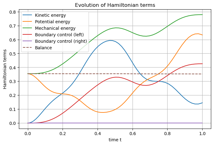
One can appreciate the structure-preserving property by looking at the dashed line, showing the evolution of

\[\mathcal{H}^d(t) - \int_0^t u_R(s) y_R(s) {\rm d}s - \int_0^t u_L(s) y_L(s) {\rm d}s.\]

And now? It is time to see more examples.