The shallow water equation

• file: examples/shallow_water.py

• authors: Ghislain Haine

• date: 22 nov. 2022

• brief: inviscid shallow water equations

examples.shallow_water.shallow_water_eq()

A structure-preserving discretization of the inviscid shallow-water equation

Formulation Grad-Grad, homogeneous boundary condition, on a tank

Setting

The objective of this example is to show how to deal with non-linearity.

Let us consider a bounded domain \(\Omega \subset \mathbb{R}^2\). The shallow water equations are constituted of two conservation laws

\[\begin{split}\begin{pmatrix} \partial_t h \\ \partial_t p \end{pmatrix} = \begin{bmatrix} 0 & - {\rm div} \\ -{\rm grad} & \frac{1}{h} G(\omega) \end{bmatrix} \begin{pmatrix} {e}_h \\ {e_p} \end{pmatrix} ,\end{split}\]

where \(h\) is the height of the fluid, \(v\) is the velocity, \(\rho\) is the fluid density (supposed constant), \(p := \rho v\) is the linear momentum, \(\omega := {\rm curl}_{2D} \left( v \right) := \partial_x v_y - \partial_y v_x\) is the vorticity, \(G(\omega):=\rho \begin{bmatrix} 0 & 1 \\ -1 & 0 \end{bmatrix}\,{\omega}\), \(e_h = \frac{1}{2} \rho\,\|v\|^2 + \rho g h\) is the total pressure and \(e_p = h v\) is the volumetric flow of the fluid. Thus, the first line of the matrix equation represents the conservation of the mass (or volume, since the fluid is assumed to be incompressible) and the second represents the conservation of linear momentum.

Port-Hamiltonian framework

One can define the system Hamiltonian (or total energy) as a functional of \(h\) and \(p\), which are thus called energy variables

\[\mathcal{H} (h,p) := \frac{1}{2} \int_\Omega \frac{h(t,x) \| p(t,x) \|^2}{\rho} + \rho g h^2(t,x) {\rm d}x.\]

The co-energy variables can be computed from the variational derivative of the Hamiltonian such that

\[\begin{split}\begin{split} e_h & = \delta_h \mathcal{H} = \frac{1}{2} \rho \| v \|^2 + \rho g h , \\ e_p & = \delta_{p} \mathcal{H} = h v . \end{split}\end{split}\]

The time-derivative of the Hamiltonian can then be obtained computed and depends only on the boundary variables

\[\frac{\rm d}{{\rm d}t} \mathcal{H} = - \int_{\partial\Omega} e_h(t,s) e_p(t,s) \cdot n(s) {\rm d}s ,\]

which enables to define collocated control and observation distributed ports along the boundary \(\partial\Omega\). For example, one may define

\[\begin{split}\begin{split} u_{\partial} & = - e_p \cdot n,\\ y_{\partial} & = e_h, \end{split}\end{split}\]

and the power-balance is given by a product between input and output boundary ports. The system is lossless, and conservative in the absence of control.

Structure-preserving discretization

First, let us multiply the linear momentum conservation equation by \(h\).

Let us consider sufficiently regular test functions \(\varphi\) and \(\Phi\) on \(\Omega\), and \(\psi\) test functions at the boundary \(\partial\Omega\). The weak form of the previous equations reads

\[\begin{split}\left\lbrace \begin{array}{rcl} \left( \partial_t h, \varphi \right)_{L^2} &=& - \left( {\rm div}\left( h e_p \right), \varphi \right)_{L^2}, \\ \left( h \partial_t p, \Phi \right)_{(L^2)^2} &=& - \left( h {\rm grad}\left( e_h \right), \Phi \right)_{(L^2)^2} + \left( {\rm curl}_{2D}\left( p \right) \begin{bmatrix} 0 & 1 \\ -1 & 0 \end{bmatrix} e_p, \Phi \right)_{(L^2)^2}, \\ \left( y_\partial, \psi \right)_{\partial\Omega} &=& \left( e_h, \psi \right)_{\partial\Omega}. \end{array} \right.\end{split}\]

Applying integration by parts on the first line leads to

\[\begin{split}\left\lbrace \begin{array}{rcl} \left( \partial_t h, \varphi \right)_{L^2} &=& \left( h e_p, {\rm grad} \left( \varphi \right) \right)_{L^2} + \left( h u_\partial, \varphi \right)_{\partial\Omega}, \\ \left( h \partial_t p, \Phi \right)_{(L^2)^2} &=& - \left( h {\rm grad} \left( e_h \right), \Phi \right)_{(L^2)^2} + \left( {\rm curl}_{2D}\left( p \right) \begin{bmatrix} 0 & 1 \\ -1 & 0 \end{bmatrix} e_p, \Phi \right)_{(L^2)^2}, \\ \left( y_\partial, \psi \right)_{\partial\Omega} &=& \left( e_h, \psi \right)_{\partial\Omega}. \end{array} \right.\end{split}\]

Furthermore, the weak form of the constitutive relations write

\[\begin{split}\left\lbrace \begin{array}{rcl} \left( e_h, \varphi \right)_{L^2} &=& \left( \rho g h, \varphi \right)_{L^2} + \left( \frac{\| p \|^2}{2 \rho}, \varphi \right)_{L^2}, \\ \left( e_p, \Phi \right)_{(L^2)^2} &=& \left( \frac{p}{\rho}, \Phi \right)_{(L^2)^2}. \end{array} \right.\end{split}\]

Now, let us choose three finite families \((\varphi^i)_{1 \le i \le N_h} \subset H^1(\Omega)\), \((\Phi^k)_{1 \le k \le N_p} \subset (L^2(\Omega))^2\) and \((\psi^m)_{1 \le m \le N_\partial}\) and project the weak formulations on them: for all \(1 \le i \le N_h\), all \(1 \le k \le N_p\) and all \(1 \le m \le N_\partial\)

\[\begin{split}\left\lbrace \begin{array}{rcl} \sum_{j=1}^{N_h} \frac{\rm d}{{\rm d}t} h^j \left( \varphi^j, \varphi^i \right)_{L^2} &=& \sum_{\ell=1}^{N_p} e_p^\ell \left( h^d \Phi^\ell, {\rm grad} \left( \varphi^i \right) \right)_{L^2} + \sum_{n=1}^{N_\partial} u_\partial^n \left( h^d \psi^n, \varphi^i \right)_{\partial\Omega}, \\ \sum_{\ell=1}^{N_p} \frac{\rm d}{{\rm d}t} p^\ell \left( h^d \Phi^\ell, \Phi^k \right)_{(L^2)^2} &=& - \sum_{j=1}^{N_h} e_h^j \left( h^d {\rm grad} \left( \varphi^j \right), \Phi^k \right)_{(L^2)^2} \\ && \quad + \sum_{\ell=1}^{N_p} e_p^\ell \left( {\rm curl}_{2D}\left( p^d \right) \begin{bmatrix} 0 & 1 \\ -1 & 0 \end{bmatrix} \Phi^\ell, \Phi^k \right)_{(L^2)^2}, \\ \sum_{n=1}^{N_\partial} y_\partial^n \left( \psi^n, \psi^m \right)_{\partial\Omega} &=& \sum_{j=1}^{N_h} e_h^j \left( \varphi^j, \psi^m \right)_{\partial\Omega}, \end{array} \right.\end{split}\]

where \(h^d := \sum_{i=1}^{N_h} h^i \varphi^i\) is the approximation of \(h\) and \(p^d := \sum_{k=1}^{N_p} p^k \Phi^k\) is the approximation of \(p\). The constitutive relations read for all \(1 \le i \le N_h\) and all \(1 \le k \le N_p\)

\[\begin{split}\left\lbrace \begin{array}{rcl} \sum_{j=1}^{N_h} e_h^j \left( \varphi^j, \varphi^i \right)_{L^2} &=& \sum_{j=1}^{N_h} h^j \left( \rho g \varphi^j, \varphi^i \right)_{L^2} + \sum_{\ell=1}^{N_p} p^\ell \left( \frac{\Phi^\ell \cdot p^d}{2 \rho}, \varphi^i \right)_{L^2}, \\ \sum_{\ell=1}^{N_p} e_p^\ell \left( \Phi^\ell, \Phi^k \right)_{(L^2)^2} &=& \sum_{\ell=1}^{N_p} p^\ell \left( \frac{\Phi^\ell}{\rho}, \Phi^k \right)_{(L^2)^2}. \end{array} \right.\end{split}\]

Defining \(\underline{\star}\) the vector gathering the coefficient of the approximation of the variable \(\star\) in its appropriate finite family, one may write the discrete weak formulations in matrix notation

\[\begin{split}\begin{bmatrix} M_h & 0 & 0 \\ 0 & M_p[h^d] & 0 \\ 0 & 0 & M_\partial \end{bmatrix} \begin{pmatrix} \underline{h} \\ \underline{p} \\ -\underline{y_\partial} \end{pmatrix} = \begin{bmatrix} 0 & D[h^d] & B[h^d] \\ -D[h^d]^\top & G[p^d] & 0 \\ - B^\top & 0 & 0 \end{bmatrix} \begin{pmatrix} \underline{e_h} \\ \underline{e_p} \\ \underline{u_\partial} \end{pmatrix}.\end{split}\]

where the matrices are given by

\[(M_h)_{ij} := \left( \varphi^j, \varphi^i \right)_{L^2} \qquad (M_p[h^d])_{k\ell} := \left( h^d \Phi^\ell, \Phi^k \right)_{(L^2)^2},\]

\[(D[h^d])_{i\ell} := \left( h^d \Phi^\ell, {\rm grad} \left( \varphi^i \right) \right)_{L^2}, \qquad (B[h^d])_{in} := \left( h^d \psi^n, \varphi^i \right)_{\partial\Omega},\]

and

\[(M_\partial)_{mn} := \left( \psi^n, \psi^m \right)_{\partial\Omega}, \qquad (B)_{in} := \left( \psi^n, \varphi^i \right)_{\partial\Omega}.\]

The constitutive relations read

\[\begin{split}\begin{bmatrix} M_h & 0 \\ 0 & M_p \end{bmatrix} \begin{pmatrix} \underline{e_h} \\ \underline{e_p} \end{pmatrix} = \begin{bmatrix} Q_h & P_h[h^d] \\ 0 & Q_p \end{bmatrix} \begin{pmatrix} \underline{h} \\ \underline{p} \end{pmatrix},\end{split}\]

where the matrices are given by

\[(M_p)_{k\ell} := \left( \Phi^\ell, \Phi^k \right)_{(L^2)^2}, \qquad (Q_h)_{ij} := \left( \rho g \varphi^j, \varphi^i \right)_{L^2},\]

\[(P_h[h^d])_{i\ell} := \left( \frac{\Phi^\ell \cdot p^d}{2 \rho}, \varphi^i \right)_{L^2}, \qquad (Q_d)_{k\ell} := \left( \frac{\Phi^\ell}{\rho}, \Phi^k \right)_{(L^2)^2}.\]

With these definition, one may prove the discrete power balance

\[\frac{\rm d}{{\rm d}t} \mathcal{H}^d(t) = \underline{u_\partial}^\top(t) M_\partial \underline{y_\partial}(t).\]

Simulation

The beggining is classical: first import, then create the dphs and set the domain.

# Import scrimp
import scrimp as S

# Init the distributed port-Hamiltonian system
swe = S.DPHS("real")

# Set the domain (using the built-in geometry `Rectangle`)
# Labels: Omega = 1, Gamma_Bottom = 10, Gamma_Right = 11, Gamma_Top = 12, Gamma_Left = 13
swe.set_domain(S.Domain("Rectangle", {"L": 2.0, "l": 0.5, "h": 0.1}))

Then the states and co-states.

# Define the states and costates
states = [
    S.State("h", "Fluid height", "scalar-field"),
    S.State("p", "Linear momentum", "vector-field"),
]
costates = [
    S.CoState("e_h", "Pressure", states[0]),
    S.CoState("e_p", "Velocity", states[1]),
]

# Add them to the dphs
for state in states:
    swe.add_state(state)
for costate in costates:
    swe.add_costate(costate)

And the control ports.

# Define the control ports
control_ports = [
    S.Control_Port(
        "Boundary control 0",
        "U_0",
        "Normal velocity",
        "Y_0",
        "Fluid height",
        "scalar-field",
        region=10,
        position="effort",
    ),
    S.Control_Port(
        "Boundary control 1",
        "U_1",
        "Normal velocity",
        "Y_1",
        "Fluid height",
        "scalar-field",
        region=11,
        position="effort",
    ),
    S.Control_Port(
        "Boundary control 2",
        "U_2",
        "Normal velocity",
        "Y_2",
        "Fluid height",
        "scalar-field",
        region=12,
        position="effort",
    ),
    S.Control_Port(
        "Boundary control 3",
        "U_3",
        "Normal velocity",
        "Y_3",
        "Fluid height",
        "scalar-field",
        region=13,
        position="effort",
    ),
]

# Add them to the dphs
for ctrl_port in control_ports:
    swe.add_control_port(ctrl_port)

Regarding the FEM, this is more challenging, as non-linearity are present. Nevertheless, let us stick to the way we choose until now: since the \(h\)-type variables will be derivated, thus we choose continuous Galerkin approximations of order \(k+1\). The other energy variable is taken as continuous Galerkin approximation of order \(k\), while boundary terms are given by discontinuous Galerkin approximations of order \(k\).

# Define the Finite Elements Method of each port
k = 1
FEMs = [
    S.FEM(states[0].get_name(), k+1, FEM="CG"),
    S.FEM(states[1].get_name(), k, FEM="CG"),
    S.FEM(control_ports[0].get_name(), k, "DG"),
    S.FEM(control_ports[1].get_name(), k, "DG"),
    S.FEM(control_ports[2].get_name(), k, "DG"),
    S.FEM(control_ports[3].get_name(), k, "DG"),
]

# Add them to the dphs
for FEM in FEMs:
    swe.add_FEM(FEM)

The parameters are physically meaningful!

# Define physical parameters
rho = 1000.
g = 10.
parameters = [
    S.Parameter("rho", "Mass density", "scalar-field", f"{rho}", "h"),
    S.Parameter("g", "Gravity", "scalar-field", f"{g}", "h"),
]

# Add them to the dphs
for parameter in parameters:
    swe.add_parameter(parameter)

Here are the difficult part. We need to define the weak form of each block matrices, and take non-linearities into account. To do so, the GFWL of GetFEM is transparent, but it is mandatory to say to SCRIMP that the Brick is non-linear, using the keyword linear=False. It is also possible to ask for this block to be considered explicitly in the time scheme (i.e. it will be computed with the previous time step values and be considered as a right-hand side), as done for the gyroscopic term below, using the keyword explicit=True.

# Define the pHs via `Brick` == non-zero block matrices == variational terms
# Some macros for the sake of readability
swe.gf_model.add_macro('div(v)', 'Trace(Grad(v))')
swe.gf_model.add_macro('Rot', '[[0,1],[-1,0]]')
swe.gf_model.add_macro('Curl2D(v)', 'div(Rot*v)')
swe.gf_model.add_macro('Gyro(v)', 'Curl2D(v)*Rot')
bricks = [
    # Define the mass matrices of the left-hand side of the "Dirac structure" (position="flow")
    S.Brick("M_h", "h * Test_h", [1], dt=True, position="flow"),
    S.Brick("M_p", "h * p . Test_p", [1], dt=True, linear=False, position="flow"),
    S.Brick("M_Y_0", "Y_0 * Test_Y_0", [10], position="flow"),
    S.Brick("M_Y_1", "Y_1 * Test_Y_1", [11], position="flow"),
    S.Brick("M_Y_2", "Y_2 * Test_Y_2", [12], position="flow"),
    S.Brick("M_Y_3", "Y_3 * Test_Y_3", [13], position="flow"),

    # Define the first line of the right-hand side of the "Dirac structure" (position="effort")
    S.Brick("-D^T", "h * e_p . Grad(Test_h)", [1], linear=False, position="effort"),
    # with the boundary control
    S.Brick("B_0", "- U_0 * Test_h", [10], position="effort"),
    S.Brick("B_1", "- U_1 * Test_h", [11], position="effort"),
    S.Brick("B_2", "- U_2 * Test_h", [12], position="effort"),
    S.Brick("B_3", "- U_3 * Test_h", [13], position="effort"),
    # Define the second line of the right-hand side of the "Dirac structure" (position="effort")
    S.Brick("D", "- Grad(e_h) . Test_p * h", [1], linear=False, position="effort"),
    # with the gyroscopic term (beware that "Curl" is not available in the GWFL of getfem)
    S.Brick("G", "(Gyro(p) * e_p) . Test_p", [1], linear=False, explicit=True, position="effort"),
    # Define the third line of the right-hand side of the "Dirac structure" (position="effort")
    S.Brick("C_0", "- e_h * Test_Y_0", [10], position="effort"),
    S.Brick("C_1", "- e_h * Test_Y_1", [11], position="effort"),
    S.Brick("C_2", "- e_h * Test_Y_2", [12], position="effort"),
    S.Brick("C_3", "- e_h * Test_Y_3", [13], position="effort"),

    ## Define the constitutive relations (position="constitutive", the default value)
    # For e_h: first the mass matrix WITH A MINUS because we want an implicit formulation 0 = - M e_h + F(h)
    S.Brick("-M_e_h", "- e_h * Test_e_h", [1]),
    # second the linear part as a linear brick
    S.Brick("Q_h", "rho * g * h * Test_e_h", [1]),
    # third the non-linear part as a non-linear brick (linear=False)
    S.Brick("P_h", "0.5 * (p . p) / rho * Test_e_h", [1], linear=False),
    # For e_p: first the mass matrix WITH A MINUS because we want an implicit formulation 0 = - M e_p + F(p)
    S.Brick("-M_e_p", "- e_p . Test_e_p", [1]),
    # second the LINEAR brick
    S.Brick("Q_p", "p / rho . Test_e_p", [1]),
]
for brick in bricks:
    swe.add_brick(brick)

As we just look at how it works, let us consider a step in the height, no initial velocity, and homogeneous Neumann boundary condition. This should look like a dam break experiment in a rectangular tank.

Remark: note the use of np, i.e. numpy, in the definition of the initial height \(h_0\).

## Initialize the problem
swe.set_control("Boundary control 0", "0.")
swe.set_control("Boundary control 1", "0.")
swe.set_control("Boundary control 2", "0.")
swe.set_control("Boundary control 3", "0.")

# Set the initial data
swe.set_initial_value("h", "3. - (np.sign(x-0.5)+1)/3.")
swe.set_initial_value("p", f"[ 0., 0.]")

## Solve in time
# Define the time scheme
swe.set_time_scheme(
    ts_type="bdf",
    ts_bdf_order=4,
    t_f=0.5,
    dt=0.0001,
    dt_save=0.01,
)

# Solve the system in time
swe.solve()

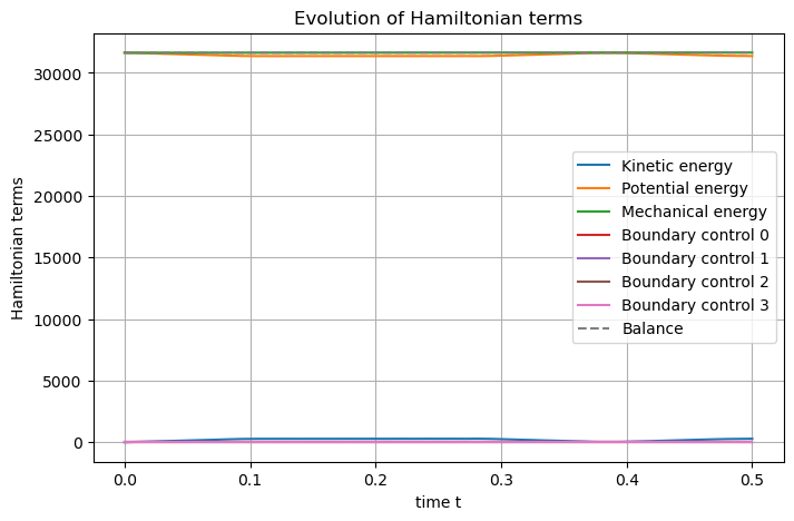
The Hamiltonian are then defined, computed, and shown.

## Post-processing
# Set Hamiltonian's name
swe.hamiltonian.set_name("Mechanical energy")
# Define Hamiltonian terms
terms = [
    S.Term("Kinetic energy", "0.5*h*p.p/rho", [1]),
    S.Term("Potential energy", "0.5*rho*g*h*h", [1]),
]
# Add them to the Hamiltonian
for term in terms:
    swe.hamiltonian.add_term(term)
# Plot the Hamiltonian
swe.plot_Hamiltonian(save_figure=True, filename="Hamiltonian_Inviscid_Shallow_Water_2D.png")