The wave equation

• file: examples/wave.py

• authors: Giuseppe Ferraro, Ghislain Haine

• date: 22 nov. 2022

• brief: 2D wave equations

examples.wave.wave_eq()

A structure-preserving discretization of the wave equation with mixed boundary control

Formulation DAE (energy/co-energy), Grad-Grad, Mixed boundary condition on the Rectangle Undamped case.

Setting

Let us consider the 2D wave equation with mixed boundary controls on a bounded rectangle \(\Omega := (0, L) \times (0, \ell)\), with boundaries \(\Gamma_N := \left( (0, L) \times \{ 0, \ell \} \right) \cup \left( \{ L \} \times (0, \ell) \right)\) and \(\Gamma_D := \{ 0 \} \times (0, \ell)\).

The deflection of the membrane from the equilibrium \(w\) satisfies classicaly

\[\begin{split}\left\lbrace \begin{array}{rcl} \rho(x) \partial_{tt}^2 w(t,x) - {\rm div} \left( T(x) \cdot {\rm grad} \left( w(t,x) \right) \right) &=& 0, \qquad t \ge 0, x \in \Omega, \\ \partial_t w(0,x) &=& v_0(x), \qquad x \in \Omega, \\ \partial_x w(0,x) &=& s_0(x), \qquad x \in \Omega, \\ T(s) \cdot {\rm grad} \left( w(t,s) \right) &=& u_N(t,s), \qquad t \ge 0, s \in \Gamma_N, \\ \partial_t w(t,s) &=& u_D(t,s), \qquad t \ge 0, s \in \Gamma_D, \end{array} \right.\end{split}\]

where \(\rho\) is the mass density and \(T\) the Young’s modulus. The subscript \(N\) stands for Neumann, while the subscript \(D\) stands for Dirichlet (to be fair, this is not really a Dirichlet boundary condition, as it imposes \(\partial_t w\) and not \(w\) at the boundary \(\Gamma_D\)).

Let us state the physics in the port-Hamiltonian formalism.

Port-Hamiltonian framework

Let \(\alpha_q := {\rm grad} w\) denotes the strain and \(\alpha_p := \rho \partial_t w\) the linear momentum. One can express the total mechanical energy lying in the system \(\mathcal{H}\), the Hamiltonian, as

\[\mathcal{H}(t) = \mathcal{H}(\alpha_q(t,x), \alpha_p(t,x)) := \underbrace{\frac{1}{2} \int_\Omega \alpha_q(t,x) \cdot T(x) \cdot \alpha_q(t,x) {\rm d}x}_{\text{Potential energy}} + \underbrace{\frac{1}{2} \int_\Omega \frac{\alpha_p(t,x)^2}{\rho(x)} {\rm d}x}_{\text{Kinetic energy}}.\]

The co-energy variables are, as in the 1D case

\[e_q := \delta_{\alpha_q} \mathcal{H} = T \cdot \alpha_q, \qquad e_p := \delta_{\alpha_p} \mathcal{H} = \frac{\alpha_p}{\rho},\]

that is the stress and the velocity respectively.

Newton’s second law and Schwarz’s lemma give the following dynamics

\[\begin{split}\begin{pmatrix} \partial_t \alpha_q \\ \partial_t \alpha_p \end{pmatrix} = \begin{bmatrix} 0 & {\rm grad} \\ {\rm div} & 0 \end{bmatrix} \begin{pmatrix} e_q \\ e_p \end{pmatrix}.\end{split}\]

Of course, this system allows to recover the initial wave equation in second-order form.

The port-Hamiltonian system representing a (linear) vibrating membrane with mixed boundary controls then writes

\[\begin{split}\begin{pmatrix} \partial_t \alpha_q \\ \partial_t \alpha_p \end{pmatrix} = \begin{bmatrix} 0 & {\rm grad} \\ {\rm div} & 0 \end{bmatrix} \begin{pmatrix} e_q \\ e_p \end{pmatrix},\end{split}\]

\[\begin{split}\left\lbrace \begin{array}{rcl} e_q(t,s) &=& u_N(t,s), \qquad t \ge 0, s \in \Gamma_N, \\ e_p(t,s) &=& u_D(t,s), \qquad t \ge 0, s \in \Gamma_D, \\ y_N(t,s) &=& e_p(t,s), \qquad t \ge 0, s \in \Gamma_N, \\ y_D(t,s) &=& e_q(t,s), \qquad t \ge 0, s \in \Gamma_D, \end{array} \right.\end{split}\]

\[\begin{split}\left\lbrace \begin{array}{rcl} e_q &=& T \cdot \alpha_q, \\ e_p &=& \frac{\alpha_p}{\rho}. \end{array} \right.\end{split}\]

The power balance satisfied by the Hamiltonian is

\[\frac{\rm d}{{\rm d}t} \mathcal{H}(t) = \underbrace{\left\langle y_N(t,\cdot), u_N(t,\cdot)\right\rangle_{\Gamma_N}}_{\text{power flowing through }\Gamma_N} + \underbrace{\left\langle u_D(t,\cdot), y_D(t,\cdot) \right\rangle_{\Gamma_D}}_{\text{power flowing through }\Gamma_D},\]

where \(\left\langle \cdot, \cdot \right\rangle_{\Gamma}\) is a boundary duality bracket \(H^\frac12, H^{-\frac12}\) at the boundary \(\Gamma\).

Structure-preserving discretization

Let \(\varphi_q\) and \(\varphi_p\) be smooth test functions on \(\Omega\), and \(\psi_N\) and \(\psi_D\) be smooth test functions on \(\Gamma_N\) and \(\Gamma_D\) respectively. One can write the weak formulation of the Dirac Structure as follows

(1)\[\begin{split} \left\lbrace \begin{array}{rcl} \int_\Omega \partial_t \alpha_q(t,x) \varphi_q(x) {\rm d}x &=& \int_\Omega {\rm grad} \left( e_p(t,x) \right) \cdot \varphi_q(x) {\rm d}x, \\ \int_\Omega \partial_t \alpha_p(t,x) \varphi_p(x) {\rm d}x &=& \int_\Omega {\rm div} \left( e_q(t,x) \right) \varphi_p(x) {\rm d}x, \\ \left\langle y_N, \psi_N \right\rangle_{\Gamma_N} &=& \left\langle e_p, \psi_N \right\rangle_{\Gamma_N}, \\ \left\langle u_D, \psi_D \right\rangle_{\Gamma_D} &=& \left\langle e_p, \psi_D \right\rangle_{\Gamma_D}. \end{array} \right.\end{split}\]

Integrating by parts the second line make the control \(u_N\) and the observation \(y_D\) appear

\[\int_\Omega \partial_t \alpha_p(t,x) \varphi_p(x) {\rm d}x = - \int_\Omega e_q(t,x) \cdot {\rm grad} \left( \varphi_p(x) \right) {\rm d}x + \left\langle \varphi_p, u_N \right\rangle_{\Gamma_N} + \left\langle \varphi_p, y_D \right\rangle_{\Gamma_D}.\]

Now, let \((\varphi_q^i)_{1 \le i \le N_q} \subset L^2(\Omega)\) and \((\varphi_p^k)_{1 \le k \le N_p} \subset H^1(\Omega)\) be two finite families of approximations for the \(q\)-type port and the \(p\)-type port respectively, typically discontinuous and continuous Galerkin finite elements respectively. Denote also \((\psi_N^m)_{1 \le m_N \le N_N} \subset H^{\frac12}(\Gamma_N)\) and \((\psi_D^m)_{1 \le m_D \le N_D} \subset H^{\frac12}(\Gamma_D)\). In particular, the latter choices imply that the duality brackets at the boundary reduce to simple \(L^2\) scalar products.

Writing the discrete weak formulation with those families, one has for all \(1 \le i \le N_q\), all \(1 \le k \le N_p\), all \(1 \le m_N \le N_N\) and all \(1 \le m_D \le N_D\)

(2)\[\begin{split} \left\lbrace \begin{array}{rcl} \sum_{j=1}^{N_q} \int_\Omega \varphi_q^j(x) \varphi_q^i(x) {\rm d}x \, \frac{\rm d}{{\rm d}t} \alpha_q^j(t) &=& \sum_{\ell=1}^{N_p} \int_\Omega {\rm grad} \left( \varphi_p^\ell(x) \right) \cdot \varphi_q^i(x) {\rm d}x \, e_p^\ell(t), \\ \sum_{\ell=1}^{N_p} \int_\Omega \varphi_p^\ell(x) \varphi_p^k(x) {\rm d}x \, \frac{\rm d}{{\rm d}t} \alpha_p^\ell(t) &=& - \sum_{j=1}^{N_q} \int_\Omega \varphi_q^j(x) \cdot {\rm grad} \left( \varphi_p^k(x) \right) {\rm d}x \, e_q^j(t) \\ && \quad + \sum_{n_N=1}^{N_N} \int_{\Gamma_N} \varphi_p^k(s) \psi_N^{n_N}(s) {\rm d}s \, u_N^{n_N}(t) \\ && \qquad + \sum_{n_D=1}^{N_D} \int_{\Gamma_D} \varphi_p^k(s) \psi_D^{n_D}(s) {\rm d}s \, y_D^{n_D}(t), \\ \sum_{n_N=1}^{N_N} \left\langle \psi_N^{n_N}, \psi_N^{m_N} \right\rangle_{\Gamma_N} \, y_N^{n_N}(t) &=& \sum_{\ell=1}^{N_p} \int_{\Gamma_N} \varphi_p^\ell(s) \psi_N^{m_N}(s) {\rm d}s \, e_p^\ell(t), \\ \sum_{n_D=1}^{N_D} \left\langle \psi_D^{n_D}, \psi_D^{m_D} \right\rangle_{\Gamma_D} \, u_D^{n_D}(t) &=& \sum_{\ell=1}^{N_p} \int_{\Gamma_D} \varphi_p^\ell(s) \psi_D^{m_D}(s) {\rm d}s \, e_p^\ell(t), \end{array} \right.\end{split}\]

which rewrites in matrix form

\[\begin{split}\underbrace{\begin{bmatrix} M_q & 0 & 0 & 0 \\ 0 & M_p & 0 & 0 \\ 0 & 0 & M_N & 0 \\ 0 & 0 & 0 & M_D \end{bmatrix}}_{= M} \begin{pmatrix} \frac{\rm d}{{\rm d}t} \underline{\alpha_q}(t) \\ \frac{\rm d}{{\rm d}t} \underline{\alpha_p}(t) \\ -\underline{y_N}(t) \\ \underline{u_D}(t) \end{pmatrix} = \underbrace{\begin{bmatrix} 0 & D & 0 & 0 \\ -D^\top & 0 & B_N & -B_D^T \\ 0 & -B_N^\top & 0 & 0 \\ 0 & B_D & 0 & 0 \end{bmatrix}}_{= J} \begin{pmatrix} \underline{e_q}(t) \\ \underline{e_p}(t) \\ \underline{u_N}(t) \\ -\underline{y_D}(t) \end{pmatrix},\end{split}\]

where \(\underline{\star}(t) := \begin{pmatrix} \star^1(t) & \cdots & \star^{N_\star} \end{pmatrix}^\top\) and

(3)\[ (M_q)_{ij} := \int_\Omega \varphi_q^j(x) \cdot \varphi_q^i(x) {\rm d}x, \qquad (M_p)_{k\ell} := \int_\Omega \varphi_p^\ell(x) \varphi_p^k(x) {\rm d}x,\]

(4)\[ (M_N)_{m_Nn_N} := \int_{\Gamma_N} \psi_N^{n_N}(s) \psi_N^{m_N}(s) {\rm d}s, \qquad (M_D)_{m_Dn_D} := \int_{\Gamma_D} \psi_D^{n_D}(s) \psi_D^{m_D}(s) {\rm d}s,\]

\[(D)_{i\ell} := \int_\Omega {\rm grad} \left( \varphi_p^\ell(x) \right) \cdot \varphi_q^i(x) {\rm d}x,\]

\[(B_N)_{n_Nk} := \int_{\Gamma_N} \varphi_p^k(s) \psi_N^{n_N}(s) {\rm d}s, \qquad (B_D)_{m_D\ell} := \int_{\Gamma_D} \varphi_p^\ell(s) \psi_D^{m_D}(s) {\rm d}s,\]

Now one can approximate the constitutive relations in those families by projection of their weak formulations

\[\begin{split}\left\lbrace \begin{array}{rcl} \int_\Omega e_q(t,x) \cdot \varphi_q(x) {\rm d}x &=& \int_\Omega \alpha_q(t,x) \cdot T(x) \cdot \varphi_q(x) {\rm d}x, \\ \int_\Omega e_p(t,x) \varphi_p(x) {\rm d}x &=& \int_\Omega \frac{\alpha_p(t,x)}{\rho(x)} \varphi_p(x) {\rm d}x, \end{array} \right.\end{split}\]

from which one can deduce the matrix form of the discrete weak formulation of the constitutive relation

\[\begin{split}\left\lbrace \begin{array}{rcl} M_q \underline{e_q}(t) &=& M_T \underline{\alpha_q}(t), \\ M_p \underline{e_p}(t) &=& M_\rho \underline{\alpha_p}(t), \end{array} \right.\end{split}\]

where

(5)\[ (M_T)_{ij} := \int_\Omega \varphi_q^j(x) \cdot T(x) \cdot \varphi_q^i(x) {\rm d}x, \qquad (M_\rho)_{k\ell} := \int_\Omega \frac{\varphi_p^\ell(x)}{\rho(x)} \varphi_p^k(x) {\rm d}x.\]

Finally, the discrete Hamiltonian \(\mathcal{H}^d\) is defined as the evaluation of \(\mathcal{H}\) on the approximation of the state variables

\[\mathcal{H}^d(t) := \mathcal{H}(\alpha_q^d(t,x), \alpha_p^d(t)) = \frac{1}{2} \underline{\alpha_q}(t)^\top M_T \underline{\alpha_q}(t) + \frac{1}{2} \underline{\alpha_p}(t)^\top M_\rho \underline{\alpha_p}(t).\]

The discrete power balance is then easily deduced from the above matrix formulations, thanks to the symmetry of \(M\) and the skew-symmetry of \(J\)

\[\frac{\rm d}{{\rm d}t} \mathcal{H}^d(t) = \underline{y_N}(t)^\top M_N \underline{u_N}(t) + \underline{u_D}(t)^\top M_D \underline{y_D}(t).\]

Simulation

Let us start by importing the scrimp package

# Import scrimp
import scrimp as S

Now define a real Distributed Port-Hamiltonian System

# Init the distributed port-Hamiltonian system
wave = S.DPHS("real")

The domain is 2-dimensional, and is a rectangle of length 2 and width 1. We use the built-in geometry Rectangle and choose a mesh size parameter of 0.1 with the following command.

# Set the domain (using the built-in geometry `Rectangle`)
# Labels: Omega = 1, Gamma_Bottom = 10, Gamma_Right = 11, Gamma_Top = 12, Gamma_Left = 13
rectangle = S.Domain("Rectangle", {"L": 2.0, "l": 1.0, "h": 0.1})

# And add it to the dphs
wave.set_domain(rectangle)

Defining the states and co-states, care must be taken: the Strain is a vector-field.

# Define the variables and their discretizations
states = [
    S.State("q", "Strain", "vector-field"),
    S.State("p", "Linear momentum", "scalar-field"),
]
costates = [
    S.CoState("e_q", "Stress", states[0]),
    S.CoState("e_p", "Velocity", states[1]),
]

# Add them to the dphs
for state in states:
    wave.add_state(state)
for costate in costates:
    wave.add_costate(costate)

As the domain is the built-in geometry Rectangle, the boundary is composed of four parts, with indices 10, 11, 12 and 13, respectively for the lower, right, upper and left edge. Each of them will have its own control port, allowing e.g. mixed boundary conditions.

Indeed in the above example, we choose Neumann boundary condition on \(\Gamma_N\), i.e. on 10, 11 and 12, while we choose Dirichlet boundary condition on \(\Gamma_D\), i.e. on 13.

The choice to integrate by part the second line of (1) has a consequence for the port at boundary 13, as it is then in the flow part of the Dirac structure, as can be seen in (2). We indicate this using the keyword position="flow".

# Define the control ports
control_ports = [
    S.Control_Port(
        "Boundary control (bottom)",
        "U_B",
        "Normal force",
        "Y_B",
        "Velocity trace",
        "scalar-field",
        region=10,
    ),
    S.Control_Port(
        "Boundary control (right)",
        "U_R",
        "Normal force",
        "Y_R",
        "Velocity trace",
        "scalar-field",
        region=11,
    ),
    S.Control_Port(
        "Boundary control (top)",
        "U_T",
        "Normal force",
        "Y_T",
        "Velocity trace",
        "scalar-field",
        region=12,
    ),
    S.Control_Port(
        "Boundary control (left)",
        "U_L",
        "Velocity trace",
        "Y_L",
        "Normal force",
        "scalar-field",
        region=13,
        position="flow",
    ),
]

# Add them to the dphs
for ctrl_port in control_ports:
    wave.add_control_port(ctrl_port)

The choice for the finite element families is often the first difficulty of a simulation. Indeed, it can result in a failing time scheme, or a very instable solution. A key-point to take a first decision is to remember which field needs regularity (in the \(L^2\)-sense) in the Dirac structure. In our case, the \(p\)-type variables should be at least \(H^1(\Omega)\), as can be inferred from (2). Hence, a first choice for the \(p\)-type variables is to take continuous Galerkin finite elements of order \(k\). Since the time derivative of \(q\) will be, more or less, a gradient of a \(p\)-type variable, it will be a discontinuous Galerkin of order \(k-1\) approximation. Finally, at least one trace of these variables, either the control, or the observation, is at most a discontinuous Galerkin of order \(k-1\) approximation. Hence the following choices, with \(k=2\).

# Define the Finite Elements Method of each port
FEMs = [
    S.FEM(states[0].get_name(), 1, "DG"),
    S.FEM(states[1].get_name(), 2, "CG"),
    S.FEM(control_ports[0].get_name(), 1, "DG"),
    S.FEM(control_ports[1].get_name(), 1, "DG"),
    S.FEM(control_ports[2].get_name(), 1, "DG"),
    S.FEM(control_ports[3].get_name(), 1, "DG"),
]

# Add them to the dphs
for FEM in FEMs:
    wave.add_FEM(FEM)

We can assume anisotropy and heterogeneity in our model by defining the parameters as follows. It has to be kept in mind that a parameter is always linked to a port (i.e., to a pair flow-effort). In particular, a parameter linked to a port that is a vector-field, should be a tensor-field.

# Define physical parameters
parameters = [
    S.Parameter("T", "Young's modulus", "tensor-field", "[[5+x,x*y],[x*y,2+y]]", "q"),
    S.Parameter("rho", "Mass density", "scalar-field", "3-x", "p"),
]

# Add them to the dphs
for parameter in parameters:
    wave.add_parameter(parameter)

It is time to define the bricks of our model, i.e. the block matrices of our discretization, providing the weak forms given in (3), (4), and (5).

This is probably the most difficult part of the process, and care must be taken. Remember that the syntax is the Generic Weak-Form Language (GWFL), for which an on-line documentation exists on the GetFEM site.

For the block matrices appearing against time derivative of a variable, it is crucial not to forget the keyword dt=True.

# Define the pHs via `Brick` == non-zero block matrices == variational terms
bricks = [
    ## Define the Dirac structure
    # Define the mass matrices from the left-hand side: the `flow` part of the Dirac structure
    S.Brick("M_q", "q.Test_q", [1], dt=True, position="flow"),
    S.Brick("M_p", "p*Test_p", [1], dt=True, position="flow"),
    S.Brick("M_Y_B", "Y_B*Test_Y_B", [10], position="flow"),
    S.Brick("M_Y_R", "Y_R*Test_Y_R", [11], position="flow"),
    S.Brick("M_Y_T", "Y_T*Test_Y_T", [12], position="flow"),
    # The Dirichlet term is applied via Lagrange multiplier == the colocated output
    S.Brick("M_Y_L", "U_L*Test_Y_L", [13], position="flow"),
    # Define the matrices from the right-hand side: the `effort` part of the Dirac structure
    S.Brick("D", "Grad(e_p).Test_q", [1], position="effort"),
    S.Brick("-D^T", "-e_q.Grad(Test_p)", [1], position="effort"),
    S.Brick("B_B", "U_B*Test_p", [10], position="effort"),
    S.Brick("B_R", "U_R*Test_p", [11], position="effort"),
    S.Brick("B_T", "U_T*Test_p", [12], position="effort"),
    # The Dirichlet term is applied via Lagrange multiplier == the colocated output
    S.Brick("B_L", "Y_L*Test_p", [13], position="effort"),
    S.Brick("C_B", "-e_p*Test_Y_B", [10], position="effort"),
    S.Brick("C_R", "-e_p*Test_Y_R", [11], position="effort"),
    S.Brick("C_T", "-e_p*Test_Y_T", [12], position="effort"),
    S.Brick("C_L", "-e_p*Test_Y_L", [13], position="effort"),
    ## Define the constitutive relations
    # Hooke's law under implicit form `- M_e_q e_q + CR_q q = 0`
    S.Brick("-M_e_q", "-e_q.Test_e_q", [1]),
    S.Brick("CR_q", "q.T.Test_e_q", [1]),
    # Linear momentum definition under implicit form `- M_e_p e_p + CR_p p = 0`
    S.Brick("-M_e_p", "-e_p*Test_e_p", [1]),
    S.Brick("CR_p", "p/rho*Test_e_p", [1]),
]

# Add all these `Bricks` to the dphs
for brick in bricks:
    wave.add_brick(brick)

The last step is to initialize the dphs, by providing the control functions and the initial values for \(q\) and \(p\) (i.e., the variables that are derivated in time in the model).

## Initialize the problem
# The controls expression, ordered as the control_ports
t_f = 5.0
expressions = ["0.", "0.", "0.", f"0.1*sin(4.*t)*sin(4*pi*y)*exp(-10.*pow((0.5*{t_f}-t),2))"]

# Add each expression to its control_port
for control_port, expression in zip(control_ports, expressions):
    # Set the control functions: it automatically constructs the related `Brick`s such that `- M_u u + f(t) = 0`
    wave.set_control(control_port.get_name(), expression)

# Set the initial data
q_0 = "[0., 0.]"
wave.set_initial_value("q", q_0)
p_0 = "3**(-20*((x-0.5)*(x-0.5)+(y-0.5)*(y-0.5)))"
wave.set_initial_value("p", p_0)

It remains to solve!

## Solve in time
# Define the time scheme ("cn" is Crank-Nicolson)
wave.set_time_scheme(ts_type="cn",
                     t_f=t_f,
                     dt_save=0.01,
                     )

# Solve
wave.solve()

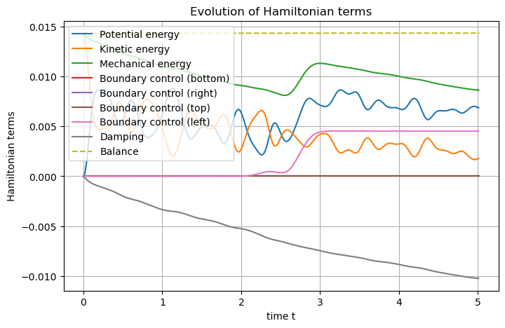
Now we can set the Hamiltonian and plot it.

## Post-processing
# Set Hamiltonian's name
wave.hamiltonian.set_name("Mechanical energy")
# Define each Hamiltonian Term
terms = [
    S.Term("Potential energy", "0.5*q.T.q", [1]),
    S.Term("Kinetic energy", "0.5*p*p/rho", [1]),
]
# Add them to the Hamiltonian
for term in terms:
    wave.hamiltonian.add_term(term)

# Plot the Hamiltonian and save the output
wave.plot_Hamiltonian(save_figure=True, filename="Hamiltonian_Wave_2D_Conservative.png")

Adding Damping to the dphs

• file: examples/wave_dissipative.py

• authors: Ghislain Haine

• date: 06 aug. 2024

• brief: 2D dissipative wave equations

examples.wave_dissipative.wave_eq()

A structure-preserving discretization of the wave equation with mixed boundary control

Formulation DAE (energy/co-energy), Grad-Grad, Mixed boundary condition on the Rectangle Damped case.

The remining part of the notebook is focused on the way to deal with dissipativity, hence using an algebraic port.

Let us come back to the continuous system. Adding a (fluid) damping consists in an additive term in Newton second law, which is proportional to the velocity (in the linear case). More precisely, denoting \(\nu\ge0\) the viscous parameter, one has:

\[\rho(x) \partial_{tt}^2 w(t,x) - {\rm div} \left( T(x) \cdot {\rm grad} \left( w(t,x) \right) \right) + \nu(x) \partial_t w(t,x) = 0.\]

Using the framework of port-Hamiltonian system, this rewrites:

\[\begin{split}\begin{pmatrix} \partial_t \alpha_q \\ \partial_t \alpha_p \end{pmatrix} = \begin{bmatrix} 0 & {\rm grad} \\ {\rm div} & 0 \end{bmatrix} \begin{pmatrix} e_q \\ e_p \end{pmatrix} + \begin{pmatrix} 0 \\ - \nu e_p \end{pmatrix}.\end{split}\]

One could include \(-\nu\) inside the matrix of operators, this is the so-called \(J-R\) framework. However, it does not exhibit the underlying Dirac structure, as it hides the resistive port. Let us introduce this hidden port, by denoting \(f_r\) the flow and \(e_r\) the effort, as follows:

(6)\[\begin{split} \begin{pmatrix} \partial_t \alpha_q \\ \partial_t \alpha_p \\ f_r \end{pmatrix} = \begin{bmatrix} 0 & {\rm grad} & 0 \\ {\rm div} & 0 & -I \\ 0 & I^\top & 0 \end{bmatrix} \begin{pmatrix} e_q \\ e_p \\ e_r \end{pmatrix},\end{split}\]

and supplemented by the resistive constitutive relation \(e_r = \nu f_r\).

Of course, at the discrete level, this will increase the number of degrees of freedom, as two extra variables have to be discretized. Nevertheless, in more complicated situations (e.g. dealing with non-linearities), this is the price to pay to recover a correct discrete power balance.

The power balance satisfied by the Hamiltonian is then

\[\frac{\rm d}{{\rm d}t} \mathcal{H}(t) = \underbrace{-\int_\Omega \nu(x) f_r^2(t,x)}_{\text{dissipated power}} \underbrace{+ \left\langle y_N(t,\cdot), u_N(t,\cdot)\right\rangle_{\Gamma_N}}_{\text{power flowing through }\Gamma_N} \underbrace{+ \left\langle u_D(t,\cdot), y_D(t,\cdot) \right\rangle_{\Gamma_D}}_{\text{power flowing through }\Gamma_D},\]

Another simulation

Let us start a new simulation with damping.

# Define a new dphs
wave_diss = S.DPHS("real")

# Set the domain (using the built-in geometry `Rectangle`)
# Labels: Omega = 1, Gamma_Bottom = 10, Gamma_Right = 11, Gamma_Top = 12, Gamma_Left = 13
rectangle = S.Domain("Rectangle", {"L": 2.0, "l": 1.0, "h": 0.1})

# On the rectangle domain
wave_diss.set_domain(rectangle)

# Define the variables
states = [
    S.State("q", "Strain", "vector-field"),
    S.State("p", "Linear momentum", "scalar-field"),
]
costates = [
    S.CoState("e_q", "Stress", states[0]),
    S.CoState("e_p", "Velocity", states[1]),
]

# Add them to the dphs
for (state,costate) in zip(states,costates):
    wave_diss.add_state(state)
    wave_diss.add_costate(costate)

# Define the control ports
control_ports = [
    S.Control_Port(
        "Boundary control (bottom)",
        "U_B",
        "Normal force",
        "Y_B",
        "Velocity trace",
        "scalar-field",
        region=10,
    ),
    S.Control_Port(
        "Boundary control (right)",
        "U_R",
        "Normal force",
        "Y_R",
        "Velocity trace",
        "scalar-field",
        region=11,
    ),
    S.Control_Port(
        "Boundary control (top)",
        "U_T",
        "Normal force",
        "Y_T",
        "Velocity trace",
        "scalar-field",
        region=12,
    ),
    S.Control_Port(
        "Boundary control (left)",
        "U_L",
        "Velocity trace",
        "Y_L",
        "Normal force",
        "scalar-field",
        region=13,
        position="flow",
    ),
]

# Add them to the dphs
for ctrl_port in control_ports:
    wave_diss.add_control_port(ctrl_port)

The additional port is defined, added to the system wave_diss and a FEM is attached to it. Remark that we use the previously defined objects, i.e. we only append the FEM of the resistive port to the list of previously defined FEM objects. We choose continuous Galerkin of order 2, as the resistive effort is of \(p\)-type.

# Define a dissipative port
port_diss = S.Port("Damping", "f_r", "e_r", "scalar-field")

# Add it to the dphs
wave_diss.add_port(port_diss)

# Define the Finite Elements Method of each port
FEMs = [
    S.FEM(states[0].get_name(), 1, "DG"),
    S.FEM(states[1].get_name(), 2, "CG"),
    S.FEM(control_ports[0].get_name(), 1, "DG"),
    S.FEM(control_ports[1].get_name(), 1, "DG"),
    S.FEM(control_ports[2].get_name(), 1, "DG"),
    S.FEM(control_ports[3].get_name(), 1, "DG"),
    S.FEM("Damping", 2, "CG"),
]

# Add all of them to the dphs
for FEM in FEMs:
    wave_diss.add_FEM(FEM)

The parameter \(\nu\) is obviously linked to the Damping port. It can be heterogeneous, as for the other parameters.

# Define physical parameters
parameters = [
    S.Parameter("T", "Young's modulus", "tensor-field", "[[5+x,x*y],[x*y,2+y]]", "q"),
    S.Parameter("rho", "Mass density", "scalar-field", "3-x", "p"),
    S.Parameter("nu", "viscosity", "scalar-field", "0.5*(2.0-x)", "Damping"),
]

# Add them to the dphs
for parameter in parameters:
    wave_diss.add_parameter(parameter)

Looking at (6), only 3 non-zero block matrices have to be added to the list of the already constructed bricks, for the Dirac structure part. And finally, 2 bricks are needed to discretize the resistive constitutive relation.

# Define the pHs via `Brick` == non-zero block matrices == variational terms
bricks = [
    ## Define the Dirac structure
    # Define the mass matrices from the left-hand side: the `flow` part of the Dirac structure
    S.Brick("M_q", "q.Test_q", [1], dt=True, position="flow"),
    S.Brick("M_p", "p*Test_p", [1], dt=True, position="flow"),
    S.Brick("M_Y_B", "Y_B*Test_Y_B", [10], position="flow"),
    S.Brick("M_Y_R", "Y_R*Test_Y_R", [11], position="flow"),
    S.Brick("M_Y_T", "Y_T*Test_Y_T", [12], position="flow"),
    # Mass matrix
    S.Brick("M_r", "f_r*Test_f_r", [1], position="flow"),
    # The Dirichlet term is applied via Lagrange multiplier == the colocated output
    S.Brick("M_Y_L", "U_L*Test_Y_L", [13], position="flow"),
    # Define the matrices from the right-hand side: the `effort` part of the Dirac structure
    S.Brick("D", "Grad(e_p).Test_q", [1], position="effort"),
    S.Brick("-D^T", "-e_q.Grad(Test_p)", [1], position="effort"),
    S.Brick("B_B", "U_B*Test_p", [10], position="effort"),
    S.Brick("B_R", "U_R*Test_p", [11], position="effort"),
    S.Brick("B_T", "U_T*Test_p", [12], position="effort"),
    # The "Identity" operator
    S.Brick("I_r", "e_r*Test_p", [1], position="effort"),
    # Minus its transpose
    S.Brick("-I_r^T", "-e_p*Test_f_r", [1], position="effort"),
    # The Dirichlet term is applied via Lagrange multiplier == the colocated output
    S.Brick("B_L", "Y_L*Test_p", [13], position="effort"),
    S.Brick("C_B", "-e_p*Test_Y_B", [10], position="effort"),
    S.Brick("C_R", "-e_p*Test_Y_R", [11], position="effort"),
    S.Brick("C_T", "-e_p*Test_Y_T", [12], position="effort"),
    S.Brick("C_L", "-e_p*Test_Y_L", [13], position="effort"),
    ## Define the constitutive relations
    # Hooke's law under implicit form `- M_e_q e_q + CR_q q = 0`
    S.Brick("-M_e_q", "-e_q.Test_e_q", [1]),
    S.Brick("CR_q", "q.T.Test_e_q", [1]),
    # Linear momentum definition under implicit form `- M_e_p e_p + CR_p p = 0`
    S.Brick("-M_e_p", "-e_p*Test_e_p", [1]),
    S.Brick("CR_p", "p/rho*Test_e_p", [1]),
    # Constitutive relation: linear viscous fluid damping `- M_e_r e_r + CR_r f_r = 0`
    S.Brick("-M_e_r", "-e_r*Test_e_r", [1]),
    S.Brick("CR_r", "nu*f_r*Test_e_r", [1]),
]

Again, we use the previsouly defined Brick objects, thus, the whole system is constructed by adding all the bricks.

# Add all these `Bricks` to the dphs
for brick in bricks:
    wave_diss.add_brick(brick)

The initialization and solve steps are identical to the previous conservative case.

## Initialize the problem
# The controls expression, ordered as the control_ports
t_f = 5.
expressions = ["0.", "0.", "0.", f"0.1*sin(4.*t)*sin(4*pi*y)*exp(-10.*pow((0.5*{t_f}-t),2))"]

# Add each expression to its control_port
for control_port, expression in zip(control_ports, expressions):
    # Set the control functions: it automatically constructs the related `Brick`s such that `- M_u u + f(t) = 0`
    wave_diss.set_control(control_port.get_name(), expression)

# Set the initial data
q_0 = "[0., 0.]"
wave_diss.set_initial_value("q", q_0)
p_0 = "3**(-20*((x-0.5)*(x-0.5)+(y-0.5)*(y-0.5)))"
wave_diss.set_initial_value("p", p_0)

## Solve in time
# Define the time scheme
wave_diss.set_time_scheme(ts_type="cn",
                          t_f=t_f,
                          dt_save=0.01,
                          )

# Solve
wave_diss.solve()

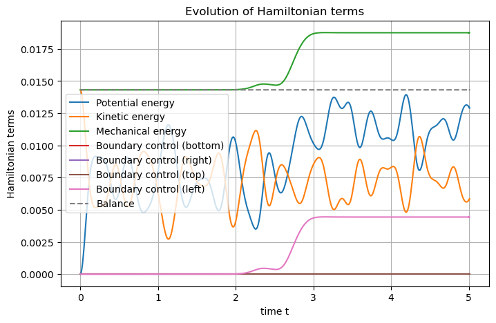
Now one can define and plot the Hamiltonian.

## Post-processing
# Set Hamiltonian's name
wave_diss.hamiltonian.set_name("Mechanical energy")

# Define each Hamiltonian Term (needed to overwrite the previously computed solution)
terms = [
    S.Term("Potential energy", "0.5*q.T.q", [1]),
    S.Term("Kinetic energy", "0.5*p*p/rho", [1]),
]

# Add them to the Hamiltonian
for term in terms:
    wave_diss.hamiltonian.add_term(term)

# Plot the Hamiltonian and save the output
wave_diss.plot_Hamiltonian(save_figure=True, filename="Hamiltonian_Wave_2D_Dissipative.png")