The heat equation
Setting
This example is the first simple case of intrinsically port-Hamiltonian Differential Algebraic Equation (known as pH-DAE).
The so-called heat equation is driven by the first law of thermodynamics.
Let \(\Omega = (0,2) \times (0,1)\) be a bounded open connected set, with mass density \(\rho(x)\), for all \(x \in \Omega\), and \(n\) be the outward unit normal at the boundary \(\partial\Omega\). We assume that:
The domain \(\Omega\) does not change over time: i.e. we work at constant volume in a solid
No chemical reaction is to be found in the domain
Dulong-Petit’s model: internal energy is proportional to temperature
Let us denotes:
\(u\) the internal energy density
\(\mathbf{J}_Q\) the heat flux
\(T\) the local temperature
\(C_V := \left( \frac{d u}{d T} \right)_V\) the isochoric heat capacity
The first law of thermodynamics, stating that in an isolated system, the energy is preserved, reads:
Under Dulong-Petit’s model, one has \(u = C_V T\), which leads to
As constitutive relation, the classical Fourier’s law is considered:
where \(\lambda\) is the tensor-valued heat conductivity of the medium.
We assume furthermore that one wants to control the temperature \(T = u_D\) at the lower, right and upper part of the boundary, denoted \(\Gamma_D\) (a Dirichlet boundary condition), while the inward heat flux \(-J_Q \cdot n = u_N\) will be prescribed at the left edge, denoted \(\Gamma_N\) (a Neumann boundary condition). Thus, the observations are \(y_D = - J_Q \cdot n\) and \(y_N = T\) respectively.
Port-Hamiltonian framework
Let us choose as Hamiltonian the usual quadratic form for parabolic equation
Computing the variational derivative with respect to the weigthed \(L^2\)-inner product \(\left( \phi, \psi \right)_\Omega := \int_\Omega \rho(x) C_V(x) \phi(x) \psi(x) {\rm d} x\) leads to a co-state variable \(e_T = T\). Hence, the first law of thermodynamics may be written as
As we want a formally skew-symmetric \(J\) operator, it has to be completed with \(-{\rm grad}\), then
and Fourier’s law provides the constitutive relation \(J_Q = \lambda f_Q\) to close the system.
Remark: \(\rho C_V\) appears against the state variable as the weight of the \(L^2\)-inner product, it should not be ommited in the mass matrix at the discrete level.
The power balance satisfied by the Hamiltonian is
where \(\left\langle \cdot, \cdot \right\rangle_{\Gamma}\) is a boundary duality bracket \(H^\frac12, H^{-\frac12}\) at the boundary \(\Gamma\).
Structure-preserving discretization
Let \(\varphi_T\) and \(\varphi_Q\) be smooth test functions on \(\Omega\), and \(\psi_N\) and \(\psi_D\) be smooth test functions on \(\Gamma_N\) and \(\Gamma_D\) respectively. One can write the weak formulation of the Dirac Structure as follows
Integrating by parts the second line make the control \(u_N\) and the observation \(y_D\) appear
Now, let \((\varphi_T^i)_{1 \le i \le N_T} \subset L^2(\Omega)\) and \((\varphi_Q^k)_{1 \le k \le N_Q} \subset H_{\rm div}(\Omega)\) be two finite families of approximations for the \(T\)-type port and the \(Q\)-type port respectively, typically discontinuous and continuous Galerkin finite elements respectively. Denote also \((\psi_N^m)_{1 \le m_N \le N_N} \subset H^{\frac12}(\Gamma_N)\) and \((\psi_D^m)_{1 \le m_N \le N_D} \subset H^{\frac12}(\Gamma_D)\). In particular, the latter choices imply that the duality brackets at the boundary reduce to simple \(L^2\) scalar products.
Writing the discrete weak formulation with those families, one has for all \(1 \le i \le N_T\), all \(1 \le k \le N_Q\), all \(1 \le m_N \le N_N\) and all \(1 \le m_D \le N_D\)
which rewrites in matrix form
where \(\underline{\star}(t) := \begin{pmatrix} \star^1(t) & \cdots & \star^{N_\star} \end{pmatrix}^\top\) and
Now one can approximate the constitutive relation
from which one can deduce the matrix form of the discrete weak formulation of the constitutive relation
where
Finally, the discrete Hamiltonian \(\mathcal{H}^d\) is defined as the evaluation of \(\mathcal{H}\) on the approximation of the state variable
The discrete power balance is then easily deduced from the above matrix formulations, thanks to the symmetry of \(M\) and the skew-symmetry of \(J\)
Simulation
As usual, we start by importing the SCRIMP package. Then we define the Distributed Port-Hamiltonian System and attach a (built-in) domain to it.
# Import scrimp
import scrimp as S

# Init the distributed port-Hamiltonian system
heat = S.DPHS("real")

# Set the domain (using the built-in geometry `Rectangle`)
# Omega = 1, Gamma_Bottom = 10, Gamma_Right = 11, Gamma_Top = 12, Gamma_Left = 13
heat.set_domain(S.Domain("Rectangle", {"L": 2.0, "l": 1.0, "h": 0.1}))
The next step is to define the state and its co-state. Care must be
taken here: both are the temperature \(T\), since the parameter
\(\rho C_V\) have been taken into account as a weight in the
\(L^2\)-inner product. Hence, one may save some computational burden
by using substituted=True which says to SCRIMP that the co-state
is substituted into the state! Only one variable is approximated and
will be computed in the sequel.
However, note that one could define a state \(e\) (namely the internal energy), and add Dulong-Petit’s law as a constitutive relation \(e = C_V T\) as usual.
# Define the variables and their discretizations and add them to the dphs
states = [
    S.State("T", "Temperature", "scalar-field"),
]
costates = [
    # Substituted=True indicates that only one variable has to be discretized on this port
    S.CoState("T", "Temperature", states[0], substituted=True)
]
Let us define the algebraic port.
ports = [
    S.Port("Heat flux", "f_Q", "J_Q", "vector-field"),
]
And finally the control ports on each of the four boundary part.
control_ports = [
    S.Control_Port(
        "Boundary control (bottom)",
        "U_B",
        "Temperature",
        "Y_B",
        "- Normal heat flux",
        "scalar-field",
        region=10,
        position="effort",
    ),
    S.Control_Port(
        "Boundary control (right)",
        "U_R",
        "Temperature",
        "Y_R",
        "- Normal heat flux",
        "scalar-field",
        region=11,
        position="effort",
    ),
    S.Control_Port(
        "Boundary control (top)",
        "U_T",
        "Temperature",
        "Y_T",
        "- Normal heat flux",
        "scalar-field",
        region=12,
        position="effort",
    ),
    S.Control_Port(
        "Boundary control (left)",
        "U_L",
        "- Normal heat flux",
        "Y_L",
        "Temperature",
        "scalar-field",
        region=13,
        position="flow",
    ),
]
Add all these objects to the DPHS.
for state in states:
    heat.add_state(state)
for costate in costates:
    heat.add_costate(costate)
for port in ports:
    heat.add_port(port)
for ctrl_port in control_ports:
    heat.add_control_port(ctrl_port)
Now, we must define the finite element families on each port. As stated in the beginning, only the :math:`varphi_Q` family needs a stronger regularity. Let us choose continuous Galerkin approximation of order 2. Then, the divergence of \(\varphi_Q\) is easily approximated by discontinuous Galerkin of order 1. At the boundary, this latter regularity will then occur, hence the choice of discontinuous Galerkin of order 1 as well.
FEMs = [
    S.FEM(states[0].get_name(), 1, FEM="DG"),
    S.FEM(ports[0].get_name(), 2, FEM="CG"),
    S.FEM(control_ports[0].get_name(), 1, FEM="DG"),
    S.FEM(control_ports[1].get_name(), 1, FEM="DG"),
    S.FEM(control_ports[2].get_name(), 1, FEM="DG"),
    S.FEM(control_ports[3].get_name(), 1, FEM="DG"),
]
for FEM in FEMs:
    heat.add_FEM(FEM)
It is now time to define the parameters, namely \(rho\), \(C_V\) and \(\lambda\). For the sake of simplicity, we assume that \(\rho\) will take \(C_V\) into account.
# Define the physical parameters
parameters = [
    S.Parameter("rho", "Mass density times heat capacity", "scalar-field", "3.", "T"),
    S.Parameter(
        "Lambda",
        "Heat conductivity",
        "tensor-field",
        "[[1e-2,0.],[0.,1e-2]]",
        "Heat flux",
    ),
]
# Add them to the dphs
for parameter in parameters:
    heat.add_parameter(parameter)
Now the non-zero block matrices of the Dirac structure can be defined
using the Brick object, as well as the constitutive relation, i.e.
Fourier’s law.
# Define the Dirac structure and the constitutive relations block matrices as `Brick`
bricks = [
    # Add the mass matrices from the left-hand side: the `flow` part of the Dirac structure
    S.Brick("M_T", "T*rho*Test_T", [1], dt=True, position="flow"),
    S.Brick("M_Q", "f_Q.Test_f_Q", [1], position="flow"),
    S.Brick("M_Y_B", "Y_B*Test_Y_B", [10], position="flow"),
    S.Brick("M_Y_R", "Y_R*Test_Y_R", [11], position="flow"),
    S.Brick("M_Y_T", "Y_T*Test_Y_T", [12], position="flow"),
    # Normal trace is imposed by Lagrange multiplier on the left side == the collocated output
    S.Brick("M_Y_L", "U_L*Test_Y_L", [13], position="flow"),
    # Add the matrices from the right-hand side: the `effort` part of the Dirac structure
    S.Brick("D", "-Div(J_Q)*Test_T", [1], position="effort"),
    S.Brick("-D^T", "T*Div(Test_f_Q)", [1], position="effort"),
    S.Brick("B_B", "-U_B*Test_f_Q.Normal", [10], position="effort"),
    S.Brick("B_R", "-U_R*Test_f_Q.Normal", [11], position="effort"),
    S.Brick("B_T", "-U_T*Test_f_Q.Normal", [12], position="effort"),
    # Normal trace is imposed by Lagrange multiplier on the left side == the collocated output
    S.Brick("B_L", "-Y_L*Test_f_Q.Normal", [13], position="effort"),
    S.Brick("C_B", "J_Q.Normal*Test_Y_B", [10], position="effort"),
    S.Brick("C_R", "J_Q.Normal*Test_Y_R", [11], position="effort"),
    S.Brick("C_T", "J_Q.Normal*Test_Y_T", [12], position="effort"),
    S.Brick("C_L", "J_Q.Normal*Test_Y_L", [13], position="effort"),
    ## Define the constitutive relations as getfem `brick`
    # Fourier's law under implicit form - M_e_Q e_Q + CR_Q Q = 0
    S.Brick("-M_J_Q", "-J_Q.Test_J_Q", [1]),
    S.Brick("CR_Q", "f_Q.Lambda.Test_J_Q", [1]),
]
for brick in bricks:
    heat.add_brick(brick)
As controls, we assume that the temperature is prescribed, while the inward heat flux is proportional to the temperature (i.e. we consider an impedance-like absorbing boundary condition). This is easily achieved in SCRIMP by calling the variable in the expression of the control to apply.
The initial temperature profile is compatible with these controls, and has a positive bump centered in the domain.
# Initialize the problem
expressions = ["1.", "1.", "1.", "0.2*T"]

for control_port, expression in zip(control_ports, expressions):
    # Set the control functions (automatic construction of bricks such that -M_u u + f(t) = 0)
    heat.set_control(control_port.get_name(), expression)

# Set the initial data
heat.set_initial_value("T", "1. + 2.*np.exp(-50*((x-1)*(x-1)+(y-0.5)*(y-0.5))**2)")
We can now solve our Differential Algebraic Equation (DAE) using, e.g., a Backward Differentiation Formula (BDF) of order 4.
## Solve in time
# Define the time scheme ("bdf" is backward differentiation formula)
heat.set_time_scheme(t_f=5.,
                     ts_type="bdf",
                     ts_bdf_order=4,
                     dt=0.01,
                     )

# Solve
heat.solve()
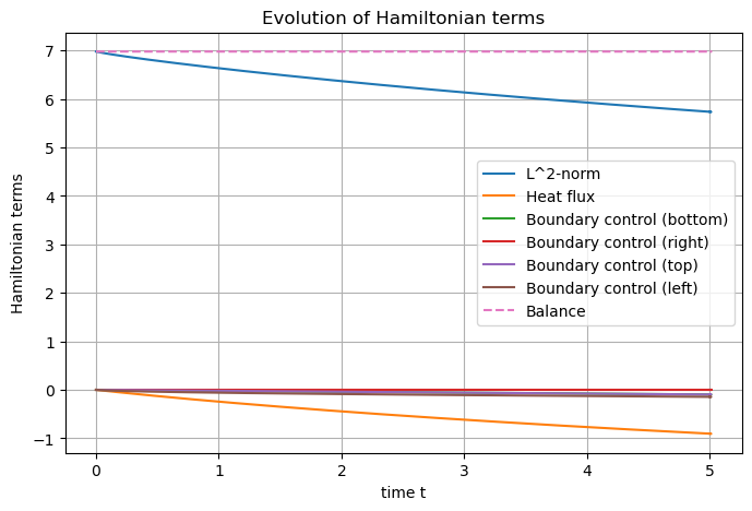
The Hamiltonian may be defined, computed and plot.
## Post-processing
# Set Hamiltonian name
heat.hamiltonian.set_name("Lyapunov formulation")
# Define the term
terms = [
    S.Term("L^2-norm", "0.5*T*rho*T", [1]),
]
# Add them to the Hamiltonian
for term in terms:
    heat.hamiltonian.add_term(term)

# Plot the Hamiltonian
heat.plot_Hamiltonian(save_figure=True, filename="Hamiltonian_Heat_2D.png")