Heat wave coupling
Setting
It is assumed that the 2D wave equation, the 2D wave equation in co-energy formulation and the 2D heat equation have already been studied.
The objective of this example is to deal with interconnection in the sense of port-Hamiltonian systems.
We are interested in the coupled heat-wave system which can be formulated as follows: let \(\Omega := \Omega_W \cup \Omega_H\) be a bounded domain in \(\mathbb{R}^2\) such that \(\Omega_W \cap \Omega_H = \emptyset\), we denote \(\Gamma_I := \partial\Omega_W \cap \partial\Omega_H\) the interface between the two domains, and \(\Gamma_W := \partial\Omega_W \setminus \Gamma_I\) and \(\Gamma_H := \partial\Omega_H \setminus \Gamma_I\). The system of equations reads
together with the transmission conditions across the interface
where \(n_H\) is the outward normal to \(\Omega_H\) and \(n_W\) is the outward normal to \(\Omega_W\). Hence, \(n_H = -n_W\) on \(\Gamma_I\).
Port-Hamiltonian framework
The heat equation
The heat equation reads
together with the boundary ports
and
The wave equation
The Dirichlet boundary condition has to be relaxed by \(\partial_t w = 0\) to fit the port-Hamiltonian framework. Providing this adaptation and the notation \(p := \partial_t w\) and \(q := {\rm grad}\left(w\right)\), the wave equation reads
together with the boundary ports
and
The interconnection
The transmission condition at the interface may be recast as a power-preserving interconnection. It can be either a gyrator or a tranformer interconnection, depending on the chosen causality for each system. We the above choices, we have a gyrator interconnection, indeed, one has
Structure-preserving discretization
The heat equation
We use the div-div formulation already presented in the 2D heat equation example, i.e. we obtain the following system
The wave equation
We use the grad-grad formulation already presented in the 2D wave equation example, i.e. we obtain the following system
The transformer interconnection
This condition is easy to implement, and leads to
Simulation
Let us start as usual, but using now the Concentric built-in
geometry.
# Import scrimp
import scrimp as S

# Init the distributed port-Hamiltonian system
hw = S.DPHS("real")

# Set the domain (using the built-in geometry `Concentric`)
# Labels: Disk = 1, Annulus = 2, Interface = 10, Boundary = 20
omega = S.Domain("Concentric", {"R": 1.0, "r": 0.6, "h": 0.1})

# And add it to the dphs
hw.set_domain(omega)
It is important to remember here one of the objective of this example:
to understand the region keyword.
For our study case, the heat equation will lie on a region
heat_region, while the wave equation will lie on another region
wave_region. And this has to be stated when defining the states and
co-states, and everytime an integral (either the weak forms or the
Hamiltonian terms) occurs.
# Define the states and costates, needs the heat and wave region's labels
heat_region = 1
wave_region = 2
states = [
    S.State("T", "Temperature", "scalar-field", region=heat_region),
    S.State("p", "Velocity", "scalar-field", region=wave_region),
    S.State("q", "Stress", "vector-field", region=wave_region),
]
# Use of the `substituted=True` keyword to get the co-energy formulation
costates = [
    S.CoState("T", "Temperature", states[0], substituted=True),
    S.CoState("p", "Velocity", states[1], substituted=True),
    S.CoState("q", "Stress", states[2], substituted=True),
]

# Add them to the dphs
for state in states:
    hw.add_state(state)
for costate in costates:
    hw.add_costate(costate)
The same is true for the resistive port for the heat equation.
# Define the algebraic port
ports = [
    S.Port("Heat flux", "e_Q", "e_Q", "vector-field", substituted=True, region=heat_region),
]

# Add it to the dphs
for port in ports:
    hw.add_port(port)

# Define the control ports
control_ports = [
    S.Control_Port(
        "Interface Heat",
        "U_T",
        "Heat flux",
        "Y_T",
        "Temperature",
        "scalar-field",
        region=10,
        position="effort"
    ),
    S.Control_Port(
        "Interface Wave",
        "U_w",
        "Velocity",
        "Y_w",
        "Velocity",
        "scalar-field",
        region=10,
        position="effort"
    ),
    # This port will be either for the wave or the heat equation
    # It corresponds to the exterior circle of radius R
    S.Control_Port(
        "Boundary",
        "U_bnd",
        "0",
        "Y_bnd",
        ".",
        "scalar-field",
        region=20,
        position="flow"
    ),
]

# Add it to the dphs
for ctrl_port in control_ports:
    hw.add_control_port(ctrl_port)
For the FEM choices, see the previous examples.
# Define the Finite Elements Method of each port
k = 1
FEMs = [
    S.FEM("T", k, "DG"),
    S.FEM("Heat flux", k+1, "CG"),
    S.FEM("Interface Heat", k, "DG"),
    S.FEM("p", k+1, "CG"),
    S.FEM("q", k, "DG"),
    S.FEM("Interface Wave", k, "DG"),
    S.FEM("Boundary", k, "DG"),
]

# Add them to the dphs
for FEM in FEMs:
    hw.add_FEM(FEM)
The Brick object does not have an optional region keyword, it
is mandatory: more precisely, it requires a list of regions as third
argument.
# Define the pHs via `Brick` == non-zero block matrices == variational terms
# Since we use co-energy formulation, constitutive relations are already taken into
# account in the mass matrices M_q and M_p
bricks = [
    # === Heat: div-div
    S.Brick("M_T", "T*Test_T", [heat_region], dt=True, position="flow"),
    S.Brick("M_Q", "e_Q.Test_e_Q", [heat_region], position="flow"),
    S.Brick("M_Y_T", "Y_T*Test_Y_T", [10], position="flow"),

    S.Brick("D_T", "-Div(e_Q)*Test_T", [heat_region], position="effort"),
    S.Brick("D_T^T", "T*Div(Test_e_Q)", [heat_region], position="effort"),
    S.Brick("B_T", "U_T*Test_e_Q.Normal", [10], position="effort"),
    S.Brick("B_T^T", "e_Q.Normal*Test_Y_T", [10], position="effort"),

    # === Wave: grad-grad
    S.Brick("M_p", "p*Test_p", [wave_region], dt=True, position="flow"),
    S.Brick("M_q", "q.Test_q", [wave_region], dt=True, position="flow"),
    S.Brick("M_Y_w", "Y_w*Test_Y_w", [10], position="flow"),

    S.Brick("D_w", "-q.Grad(Test_p)", [wave_region], position="effort"),
    S.Brick("-D_w^T", "Grad(p).Test_q", [wave_region], position="effort"),
    S.Brick("B_w", "U_w*Test_p", [10], position="effort"),
    S.Brick("B_w^T", "p*Test_Y_w", [10], position="effort"),
]
# === Boundary depends on where is the heat equation / wave equation
if wave_region==1:
    bricks.append(S.Brick("M_Y_bnd", "Y_bnd*Test_Y_bnd", [20], position="flow"))
    bricks.append(S.Brick("B_bnd", "U_bnd*Test_e_Q.Normal", [20], position="effort"))
    bricks.append(S.Brick("B_bnd^T", "e_Q.Normal*Test_Y_bnd", [20], position="effort"))
else:
    bricks.append(S.Brick("M_Y_bnd", "U_bnd*Test_Y_bnd", [20], position="flow"))
    bricks.append(S.Brick("B_bnd", "Y_bnd*Test_p", [20], position="effort"))
    bricks.append(S.Brick("B_bnd^T", "p*Test_Y_bnd", [20], position="effort"))
for brick in bricks:
    hw.add_brick(brick)
Finally, the gyrator interconnection for a system is just an output feedback from the other. The subtility is that, while the normal along \(\Gamma_I\) depends from which side it is computed on paper, this is not the case numerically: a minus sign is necessary.
# Set the controls
# === Gyrator interconnection
hw.set_control("Interface Heat", "Y_w")
# CAREFUL: the numerical normal is the same for both sub-domains! Hence the minus sign.
hw.set_control("Interface Wave", "-Y_T")
# === Dirichlet boundary condition
hw.set_control("Boundary", "0.")

# Set the initial data
hw.set_initial_value("T", "5.*np.exp(-25*((x-0.6)*(x-0.6)+y*y))")
hw.set_initial_value("p", "5.*np.exp(-25*((x-0.6)*(x-0.6)+y*y))")
hw.set_initial_value("q", "[0.,0.]")

## Solve in time
# Define the time scheme ("bdf" is backward differentiation formula)
hw.set_time_scheme(ts_type="bdf",
                   t_f=15.,
                   dt=0.001,
                   dt_save=0.05,
                   ksp_type="preonly",
                   pc_type="lu",
                   pc_factor_mat_solver_type="mumps",
                   )

# Solve
hw.solve()
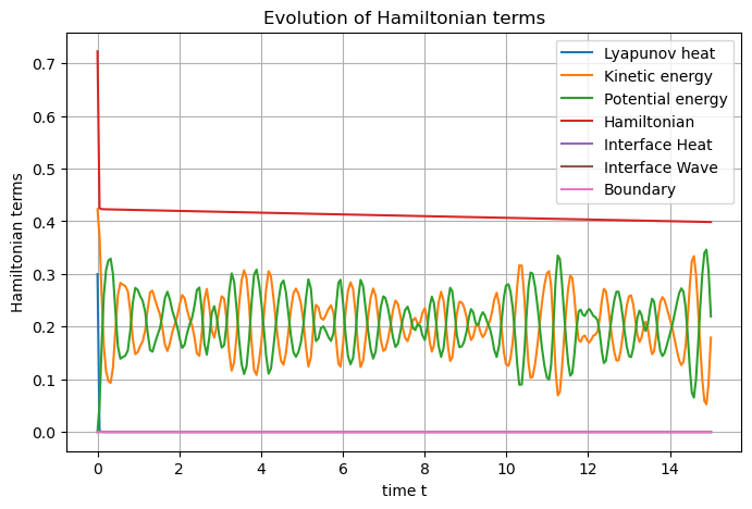
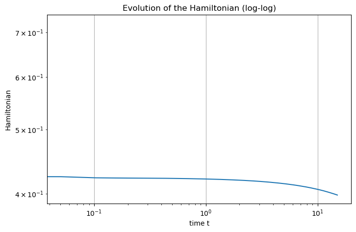
We end as usual with the Hamiltonian plot. Since our study case is known
to be strongly stable, but never exponential nor uniformly in the
initial state, we may also invocate the get_Hamiltonian method to
make a log-log view of its evolution.
## Post-processing
## Set Hamiltonian's name
hw.hamiltonian.set_name("Hamiltonian")
# Define each Hamiltonian Term
terms = [
    S.Term("Lyapunov heat", "0.5*T*T", [heat_region]),
    S.Term("Kinetic energy", "0.5*p*p", [wave_region]),
    S.Term("Potential energy", "0.5*q.q", [wave_region]),
]
# Add them to the Hamiltonian
for term in terms:
    hw.hamiltonian.add_term(term)

# Plot the Hamiltonian and save the output
hw.plot_Hamiltonian(save_figure=True, filename="Hamiltonian_Heat"+str(heat_region)+"_Wave"+str(wave_region)+"_2D.png")

# Plot the Hamiltonian in log-log scale
t = hw.solution["t"]
Hamiltonian = hw.get_Hamiltonian()
import matplotlib.pyplot as plt
fig = plt.figure(figsize=[8, 5])
ax = fig.add_subplot(111)
ax.loglog(t, Hamiltonian)
ax.grid(axis="both")
ax.set_xlabel("time t")
ax.set_ylabel("Hamiltonian")
ax.set_title("Evolution of the Hamiltonian (log-log)")
plt.show()